Modeling a Pin-Cell
This notebook is intended to demonstrate the basic features of the Python API for constructing input files and running OpenMC. In it, we will show how to create a basic reflective pin-cell model that is equivalent to modeling an infinite array of fuel pins. If you have never used OpenMC, this can serve as a good starting point to learn the Python API. We highly recommend having a copy of the Python API reference documentation open in another browser tab that you can refer to.
[1]:
%matplotlib inline
import openmc
Defining Materials
Materials in OpenMC are defined as a set of nuclides with specified atom/weight fractions. To begin, we will create a material by making an instance of the Material class. In OpenMC, many objects, including materials, are identified by a “unique ID” that is simply just a positive integer. These IDs are used when exporting XML files that the solver reads in. They also appear in the output and can be used for identification. Since an integer ID is not very useful by itself, you can also give a
material a name as well.
[2]:
uo2 = openmc.Material(1, "uo2")
print(uo2)
Material
        ID             =        1
        Name           =        uo2
        Temperature    =        None
        Density        =        None [sum]
        S(a,b) Tables
        Nuclides
On the XML side, you have no choice but to supply an ID. However, in the Python API, if you don’t give an ID, one will be automatically generated for you:
[3]:
mat = openmc.Material()
print(mat)
Material
        ID             =        2
        Name           =
        Temperature    =        None
        Density        =        None [sum]
        S(a,b) Tables
        Nuclides
We see that an ID of 2 was automatically assigned. Let’s now move on to adding nuclides to our uo2 material. The Material object has a method add_nuclide() whose first argument is the name of the nuclide and second argument is the atom or weight fraction.
[4]:
help(uo2.add_nuclide)
Help on method add_nuclide in module openmc.material:

add_nuclide(nuclide, percent, percent_type='ao') method of openmc.material.Material instance
    Add a nuclide to the material

    Parameters
    ----------
    nuclide : str
        Nuclide to add, e.g., 'Mo95'
    percent : float
        Atom or weight percent
    percent_type : {'ao', 'wo'}
        'ao' for atom percent and 'wo' for weight percent
We see that by default it assumes we want an atom fraction.
[5]:
# Add nuclides to uo2
uo2.add_nuclide('U235', 0.03)
uo2.add_nuclide('U238', 0.97)
uo2.add_nuclide('O16', 2.0)
Now we need to assign a total density to the material. We’ll use the set_density for this.
[6]:
uo2.set_density('g/cm3', 10.0)
You may sometimes be given a material specification where all the nuclide densities are in units of atom/b-cm. In this case, you just want the density to be the sum of the constituents. In that case, you can simply run mat.set_density('sum').
With UO2 finished, let’s now create materials for the clad and coolant. Note the use of add_element() for zirconium.
[7]:
zirconium = openmc.Material(name="zirconium")
zirconium.add_element('Zr', 1.0)
zirconium.set_density('g/cm3', 6.6)

water = openmc.Material(name="h2o")
water.add_nuclide('H1', 2.0)
water.add_nuclide('O16', 1.0)
water.set_density('g/cm3', 1.0)
An astute observer might now point out that this water material we just created will only use free-atom cross sections. We need to tell it to use an \(S(\alpha,\beta)\) table so that the bound atom cross section is used at thermal energies. To do this, there’s an add_s_alpha_beta() method. Note the use of the GND-style name “c_H_in_H2O”.
[8]:
water.add_s_alpha_beta('c_H_in_H2O')
When we go to run the transport solver in OpenMC, it is going to look for a materials.xml file. Thus far, we have only created objects in memory. To actually create a materials.xml file, we need to instantiate a Materials collection and export it to XML.
[9]:
materials = openmc.Materials([uo2, zirconium, water])
Note that Materials is actually a subclass of Python’s built-in list, so we can use methods like append(), insert(), pop(), etc.
[10]:
materials = openmc.Materials()
materials.append(uo2)
materials += [zirconium, water]
isinstance(materials, list)
[10]:
True
Finally, we can create the XML file with the export_to_xml() method. In a Jupyter notebook, we can run a shell command by putting ! before it, so in this case we are going to display the materials.xml file that we created.
[11]:
materials.export_to_xml()
!cat materials.xml
<?xml version='1.0' encoding='utf-8'?>
<materials>
  <material depletable="true" id="1" name="uo2">
    <density units="g/cm3" value="10.0" />
    <nuclide ao="0.03" name="U235" />
    <nuclide ao="0.97" name="U238" />
    <nuclide ao="2.0" name="O16" />
  </material>
  <material id="3" name="zirconium">
    <density units="g/cm3" value="6.6" />
    <nuclide ao="0.5145" name="Zr90" />
    <nuclide ao="0.1122" name="Zr91" />
    <nuclide ao="0.1715" name="Zr92" />
    <nuclide ao="0.1738" name="Zr94" />
    <nuclide ao="0.028" name="Zr96" />
  </material>
  <material id="4" name="h2o">
    <density units="g/cm3" value="1.0" />
    <nuclide ao="2.0" name="H1" />
    <nuclide ao="1.0" name="O16" />
    <sab name="c_H_in_H2O" />
  </material>
</materials>
Element Expansion
Did you notice something really cool that happened to our Zr element? OpenMC automatically turned it into a list of nuclides when it exported it! The way this feature works is as follows:
- First, it checks whether
Materials.cross_sectionshas been set, indicating the path to across_sections.xmlfile. - If
Materials.cross_sectionsisn’t set, it looks for theOPENMC_CROSS_SECTIONSenvironment variable. - If either of these are found, it scans the file to see what nuclides are actually available and will expand elements accordingly.
Let’s see what happens if we change O16 in water to elemental O.
[12]:
water.remove_nuclide('O16')
water.add_element('O', 1.0)

materials.export_to_xml()
!cat materials.xml
<?xml version='1.0' encoding='utf-8'?>
<materials>
  <material depletable="true" id="1" name="uo2">
    <density units="g/cm3" value="10.0" />
    <nuclide ao="0.03" name="U235" />
    <nuclide ao="0.97" name="U238" />
    <nuclide ao="2.0" name="O16" />
  </material>
  <material id="3" name="zirconium">
    <density units="g/cm3" value="6.6" />
    <nuclide ao="0.5145" name="Zr90" />
    <nuclide ao="0.1122" name="Zr91" />
    <nuclide ao="0.1715" name="Zr92" />
    <nuclide ao="0.1738" name="Zr94" />
    <nuclide ao="0.028" name="Zr96" />
  </material>
  <material id="4" name="h2o">
    <density units="g/cm3" value="1.0" />
    <nuclide ao="2.0" name="H1" />
    <nuclide ao="0.999621" name="O16" />
    <nuclide ao="0.000379" name="O17" />
    <sab name="c_H_in_H2O" />
  </material>
</materials>
We see that now O16 and O17 were automatically added. O18 is missing because our cross sections file (which is based on ENDF/B-VII.1) doesn’t have O18. If OpenMC didn’t know about the cross sections file, it would have assumed that all isotopes exist.
The cross_sections.xml file
The cross_sections.xml tells OpenMC where it can find nuclide cross sections and \(S(\alpha,\beta)\) tables. It serves the same purpose as MCNP’s xsdir file and Serpent’s xsdata file. As we mentioned, this can be set either by the OPENMC_CROSS_SECTIONS environment variable or the Materials.cross_sections attribute.
Let’s have a look at what’s inside this file:
[13]:
!cat $OPENMC_CROSS_SECTIONS | head -n 10
print('    ...')
!cat $OPENMC_CROSS_SECTIONS | tail -n 10
<?xml version='1.0' encoding='utf-8'?>
<cross_sections>
  <library materials="H1" path="H1.h5" type="neutron" />
  <library materials="H2" path="H2.h5" type="neutron" />
  <library materials="H3" path="H3.h5" type="neutron" />
  <library materials="He3" path="He3.h5" type="neutron" />
  <library materials="He4" path="He4.h5" type="neutron" />
  <library materials="Li6" path="Li6.h5" type="neutron" />
  <library materials="Li7" path="Li7.h5" type="neutron" />
  <library materials="Be7" path="Be7.h5" type="neutron" />
    ...
  <library materials="Cf253" path="wmp/098253.h5" type="wmp" />
  <library materials="Cf254" path="wmp/098254.h5" type="wmp" />
  <library materials="Es251" path="wmp/099251.h5" type="wmp" />
  <library materials="Es252" path="wmp/099252.h5" type="wmp" />
  <library materials="Es253" path="wmp/099253.h5" type="wmp" />
  <library materials="Es254" path="wmp/099254.h5" type="wmp" />
  <library materials="Es254_m1" path="wmp/099254m1.h5" type="wmp" />
  <library materials="Es255" path="wmp/099255.h5" type="wmp" />
  <library materials="Fm255" path="wmp/100255.h5" type="wmp" />
</cross_sections>
Enrichment
Note that the add_element() method has a special argument enrichment that can be used for Uranium. For example, if we know that we want to create 3% enriched UO2, the following would work:
[14]:
uo2_three = openmc.Material()
uo2_three.add_element('U', 1.0, enrichment=3.0)
uo2_three.add_element('O', 2.0)
uo2_three.set_density('g/cc', 10.0)
Mixtures
In OpenMC it is also possible to define materials by mixing existing materials. For example, if we wanted to create MOX fuel out of a mixture of UO2 (97 wt%) and PuO2 (3 wt%) we could do the following:
[15]:
# Create PuO2 material
puo2 = openmc.Material()
puo2.add_nuclide('Pu239', 0.94)
puo2.add_nuclide('Pu240', 0.06)
puo2.add_nuclide('O16', 2.0)
puo2.set_density('g/cm3', 11.5)

# Create the mixture
mox = openmc.Material.mix_materials([uo2, puo2], [0.97, 0.03], 'wo')
The ‘wo’ argument in the mix_materials() method specifies that the fractions are weight fractions. Materials can also be mixed by atomic and volume fractions with ‘ao’ and ‘vo’, respectively. For ‘ao’ and ‘wo’ the fractions must sum to one. For ‘vo’, if fractions do not sum to one, the remaining fraction is set as void.
Defining Geometry
At this point, we have three materials defined, exported to XML, and ready to be used in our model. To finish our model, we need to define the geometric arrangement of materials. OpenMC represents physical volumes using constructive solid geometry (CSG), also known as combinatorial geometry. The object that allows us to assign a material to a region of space is called a Cell (same concept in MCNP, for those familiar). In order to define a region that we can assign to a cell, we must first
define surfaces which bound the region. A surface is a locus of zeros of a function of Cartesian coordinates \(x\), \(y\), and \(z\), e.g.
- A plane perpendicular to the x axis: \(x - x_0 = 0\)
- A cylinder parallel to the z axis: \((x - x_0)^2 + (y - y_0)^2 - R^2 = 0\)
- A sphere: \((x - x_0)^2 + (y - y_0)^2 + (z - z_0)^2 - R^2 = 0\)
Between those three classes of surfaces (planes, cylinders, spheres), one can construct a wide variety of models. It is also possible to define cones and general second-order surfaces (tori are not currently supported).
Note that defining a surface is not sufficient to specify a volume – in order to define an actual volume, one must reference the half-space of a surface. A surface half-space is the region whose points satisfy a positive or negative inequality of the surface equation. For example, for a sphere of radius one centered at the origin, the surface equation is \(f(x,y,z) = x^2 + y^2 + z^2 - 1 = 0\). Thus, we say that the negative half-space of the sphere, is defined as the collection of points satisfying \(f(x,y,z) < 0\), which one can reason is the inside of the sphere. Conversely, the positive half-space of the sphere would correspond to all points outside of the sphere.
Let’s go ahead and create a sphere and confirm that what we’ve told you is true.
[16]:
sphere = openmc.Sphere(r=1.0)
Note that by default the sphere is centered at the origin so we didn’t have to supply x0, y0, or z0 arguments. Strictly speaking, we could have omitted R as well since it defaults to one. To get the negative or positive half-space, we simply need to apply the - or + unary operators, respectively.
(NOTE: Those unary operators are defined by special methods: __pos__ and __neg__ in this case).
[17]:
inside_sphere = -sphere
outside_sphere = +sphere
Now let’s see if inside_sphere actually contains points inside the sphere:
[18]:
print((0,0,0) in inside_sphere, (0,0,2) in inside_sphere)
print((0,0,0) in outside_sphere, (0,0,2) in outside_sphere)
True False
False True
Everything works as expected! Now that we understand how to create half-spaces, we can create more complex volumes by combining half-spaces using Boolean operators: & (intersection), | (union), and ~ (complement). For example, let’s say we want to define a region that is the top part of the sphere (all points inside the sphere that have \(z > 0\).
[19]:
z_plane = openmc.ZPlane(z0=0)
northern_hemisphere = -sphere & +z_plane
For many regions, OpenMC can automatically determine a bounding box. To get the bounding box, we use the bounding_box property of a region, which returns a tuple of the lower-left and upper-right Cartesian coordinates for the bounding box:
[20]:
northern_hemisphere.bounding_box
[20]:
(array([-1., -1., 0.]), array([1., 1., 1.]))
Now that we see how to create volumes, we can use them to create a cell.
[21]:
cell = openmc.Cell()
cell.region = northern_hemisphere

# or...
cell = openmc.Cell(region=northern_hemisphere)
By default, the cell is not filled by any material (void). In order to assign a material, we set the fill property of a Cell.
[22]:
cell.fill = water
Universes and in-line plotting
A collection of cells is known as a universe (again, this will be familiar to MCNP/Serpent users) and can be used as a repeatable unit when creating a model. Although we don’t need it yet, the benefit of creating a universe is that we can visualize our geometry while we’re creating it.
[23]:
universe = openmc.Universe()
universe.add_cell(cell)

# this also works
universe = openmc.Universe(cells=[cell])
The Universe object has a plot method that will display our the universe as current constructed:
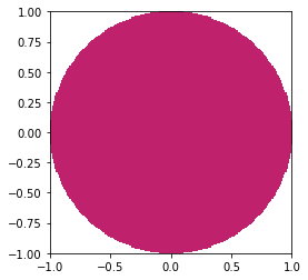
[24]:
universe.plot(width=(2.0, 2.0))
[24]:
<matplotlib.image.AxesImage at 0x7f7df827b250>
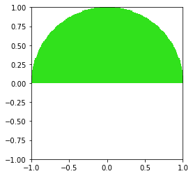
By default, the plot will appear in the \(x\)-\(y\) plane. We can change that with the basis argument.
[25]:
universe.plot(width=(2.0, 2.0), basis='xz')
[25]:
<matplotlib.image.AxesImage at 0x7f7df8112100>
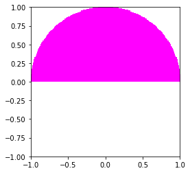
If we have particular fondness for, say, fuchsia, we can tell the plot() method to make our cell that color.
[26]:
universe.plot(width=(2.0, 2.0), basis='xz',
              colors={cell: 'fuchsia'})
[26]:
<matplotlib.image.AxesImage at 0x7f7df80edd30>
Pin cell geometry
We now have enough knowledge to create our pin-cell. We need three surfaces to define the fuel and clad:
- The outer surface of the fuel – a cylinder parallel to the z axis
- The inner surface of the clad – same as above
- The outer surface of the clad – same as above
These three surfaces will all be instances of openmc.ZCylinder, each with a different radius according to the specification.
[27]:
fuel_outer_radius = openmc.ZCylinder(r=0.39)
clad_inner_radius = openmc.ZCylinder(r=0.40)
clad_outer_radius = openmc.ZCylinder(r=0.46)
With the surfaces created, we can now take advantage of the built-in operators on surfaces to create regions for the fuel, the gap, and the clad:
[28]:
fuel_region = -fuel_outer_radius
gap_region = +fuel_outer_radius & -clad_inner_radius
clad_region = +clad_inner_radius & -clad_outer_radius
Now we can create corresponding cells that assign materials to these regions. As with materials, cells have unique IDs that are assigned either manually or automatically. Note that the gap cell doesn’t have any material assigned (it is void by default).
[29]:
fuel = openmc.Cell(name='fuel')
fuel.fill = uo2
fuel.region = fuel_region

gap = openmc.Cell(name='air gap')
gap.region = gap_region

clad = openmc.Cell(name='clad')
clad.fill = zirconium
clad.region = clad_region
Finally, we need to handle the coolant outside of our fuel pin. To do this, we create x- and y-planes that bound the geometry.
[30]:
pitch = 1.26
left = openmc.XPlane(x0=-pitch/2, boundary_type='reflective')
right = openmc.XPlane(x0=pitch/2, boundary_type='reflective')
bottom = openmc.YPlane(y0=-pitch/2, boundary_type='reflective')
top = openmc.YPlane(y0=pitch/2, boundary_type='reflective')
The water region is going to be everything outside of the clad outer radius and within the box formed as the intersection of four half-spaces.
[31]:
water_region = +left & -right & +bottom & -top & +clad_outer_radius

moderator = openmc.Cell(name='moderator')
moderator.fill = water
moderator.region = water_region
OpenMC also includes a factory function that generates a rectangular prism that could have made our lives easier.
[32]:
box = openmc.rectangular_prism(width=pitch, height=pitch,
                               boundary_type='reflective')
type(box)
[32]:
openmc.region.Intersection
Pay attention here – the object that was returned is NOT a surface. It is actually the intersection of four surface half-spaces, just like we created manually before. Thus, we don’t need to apply the unary operator (-box). Instead, we can directly combine it with +clad_or.
[33]:
water_region = box & +clad_outer_radius
The final step is to assign the cells we created to a universe and tell OpenMC that this universe is the “root” universe in our geometry. The Geometry is the final object that is actually exported to XML.
[34]:
root_universe = openmc.Universe(cells=(fuel, gap, clad, moderator))

geometry = openmc.Geometry()
geometry.root_universe = root_universe

# or...
geometry = openmc.Geometry(root_universe)
geometry.export_to_xml()
!cat geometry.xml
<?xml version='1.0' encoding='utf-8'?>
<geometry>
  <cell id="3" material="1" name="fuel" region="-3" universe="3" />
  <cell id="4" material="void" name="air gap" region="3 -4" universe="3" />
  <cell id="5" material="3" name="clad" region="4 -5" universe="3" />
  <cell id="6" material="4" name="moderator" region="6 -7 8 -9 5" universe="3" />
  <surface coeffs="0.0 0.0 0.39" id="3" type="z-cylinder" />
  <surface coeffs="0.0 0.0 0.4" id="4" type="z-cylinder" />
  <surface coeffs="0.0 0.0 0.46" id="5" type="z-cylinder" />
  <surface boundary="reflective" coeffs="-0.63" id="6" type="x-plane" />
  <surface boundary="reflective" coeffs="0.63" id="7" type="x-plane" />
  <surface boundary="reflective" coeffs="-0.63" id="8" type="y-plane" />
  <surface boundary="reflective" coeffs="0.63" id="9" type="y-plane" />
</geometry>
Starting source and settings
The Python API has a module openmc.stats with various univariate and multivariate probability distributions. We can use these distributions to create a starting source using the openmc.Source object.
[35]:
# Create a point source
point = openmc.stats.Point((0, 0, 0))
source = openmc.Source(space=point)
Now let’s create a Settings object and give it the source we created along with specifying how many batches and particles we want to run.
[36]:
settings = openmc.Settings()
settings.source = source
settings.batches = 100
settings.inactive = 10
settings.particles = 1000
[37]:
settings.export_to_xml()
!cat settings.xml
<?xml version='1.0' encoding='utf-8'?>
<settings>
  <run_mode>eigenvalue</run_mode>
  <particles>1000</particles>
  <batches>100</batches>
  <inactive>10</inactive>
  <source strength="1.0">
    <space type="point">
      <parameters>0 0 0</parameters>
    </space>
  </source>
</settings>
User-defined tallies
We actually have all the required files needed to run a simulation. Before we do that though, let’s give a quick example of how to create tallies. We will show how one would tally the total, fission, absorption, and (n,:math:gamma) reaction rates for \(^{235}\)U in the cell containing fuel. Recall that filters allow us to specify where in phase-space we want events to be tallied and scores tell us what we want to tally:
In this case, the where is “the fuel cell”. So, we will create a cell filter specifying the fuel cell.
[38]:
cell_filter = openmc.CellFilter(fuel)

tally = openmc.Tally(1)
tally.filters = [cell_filter]
The what is the total, fission, absorption, and (n,:math:gamma) reaction rates in \(^{235}\)U. By default, if we only specify what reactions, it will gives us tallies over all nuclides. We can use the nuclides attribute to name specific nuclides we’re interested in.
[39]:
tally.nuclides = ['U235']
tally.scores = ['total', 'fission', 'absorption', '(n,gamma)']
Similar to the other files, we need to create a Tallies collection and export it to XML.
[40]:
tallies = openmc.Tallies([tally])
tallies.export_to_xml()
!cat tallies.xml
<?xml version='1.0' encoding='utf-8'?>
<tallies>
  <filter id="1" type="cell">
    <bins>3</bins>
  </filter>
  <tally id="1">
    <filters>1</filters>
    <nuclides>U235</nuclides>
    <scores>total fission absorption (n,gamma)</scores>
  </tally>
</tallies>
Running OpenMC
Running OpenMC from Python can be done using the openmc.run() function. This function allows you to set the number of MPI processes and OpenMP threads, if need be.
[41]:
openmc.run()
                                %%%%%%%%%%%%%%%
                           %%%%%%%%%%%%%%%%%%%%%%%%
                        %%%%%%%%%%%%%%%%%%%%%%%%%%%%%%
                      %%%%%%%%%%%%%%%%%%%%%%%%%%%%%%%%%%
                    %%%%%%%%%%%%%%%%%%%%%%%%%%%%%%%%%%%%%%
                   %%%%%%%%%%%%%%%%%%%%%%%%%%%%%%%%%%%%%%%%
                                    %%%%%%%%%%%%%%%%%%%%%%%%
                                     %%%%%%%%%%%%%%%%%%%%%%%%
                 ###############      %%%%%%%%%%%%%%%%%%%%%%%%
                ##################     %%%%%%%%%%%%%%%%%%%%%%%
                ###################     %%%%%%%%%%%%%%%%%%%%%%%
                ####################     %%%%%%%%%%%%%%%%%%%%%%
                #####################     %%%%%%%%%%%%%%%%%%%%%
                ######################     %%%%%%%%%%%%%%%%%%%%
                #######################     %%%%%%%%%%%%%%%%%%
                 #######################     %%%%%%%%%%%%%%%%%
                 ######################     %%%%%%%%%%%%%%%%%
                  ####################     %%%%%%%%%%%%%%%%%
                    #################     %%%%%%%%%%%%%%%%%
                     ###############     %%%%%%%%%%%%%%%%
                       ############     %%%%%%%%%%%%%%%
                          ########     %%%%%%%%%%%%%%
                                      %%%%%%%%%%%

                   | The OpenMC Monte Carlo Code
         Copyright | 2011-2020 MIT and OpenMC contributors
           License | https://docs.openmc.org/en/latest/license.html
           Version | 0.12.0
          Git SHA1 | 3d90a9f857ec72eae897e054d4225180f1fa4d93
         Date/Time | 2020-08-25 14:58:51
    OpenMP Threads | 4

 Reading settings XML file...
 Reading cross sections XML file...
 Reading materials XML file...
 Reading geometry XML file...
 Reading U235 from /home/master/data/nuclear/endfb71_hdf5/U235.h5
 Reading U238 from /home/master/data/nuclear/endfb71_hdf5/U238.h5
 Reading O16 from /home/master/data/nuclear/endfb71_hdf5/O16.h5
 Reading Zr90 from /home/master/data/nuclear/endfb71_hdf5/Zr90.h5
 Reading Zr91 from /home/master/data/nuclear/endfb71_hdf5/Zr91.h5
 Reading Zr92 from /home/master/data/nuclear/endfb71_hdf5/Zr92.h5
 Reading Zr94 from /home/master/data/nuclear/endfb71_hdf5/Zr94.h5
 Reading Zr96 from /home/master/data/nuclear/endfb71_hdf5/Zr96.h5
 Reading H1 from /home/master/data/nuclear/endfb71_hdf5/H1.h5
 Reading O17 from /home/master/data/nuclear/endfb71_hdf5/O17.h5
 Reading c_H_in_H2O from /home/master/data/nuclear/endfb71_hdf5/c_H_in_H2O.h5
 Minimum neutron data temperature: 294.000000 K
 Maximum neutron data temperature: 294.000000 K
 Reading tallies XML file...
 Preparing distributed cell instances...
 Writing summary.h5 file...
 Maximum neutron transport energy: 20000000.000000 eV for U235
 Initializing source particles...

 ====================>     K EIGENVALUE SIMULATION     <====================

  Bat./Gen.      k            Average k
  =========   ========   ====================
        1/1    1.42066
        2/1    1.39831
        3/1    1.46207
        4/1    1.44888
        5/1    1.42595
        6/1    1.35549
        7/1    1.36717
        8/1    1.45095
        9/1    1.36061
       10/1    1.36554
       11/1    1.36973
       12/1    1.44276    1.40625 +/- 0.03652
       13/1    1.35512    1.38920 +/- 0.02711
       14/1    1.54216    1.42744 +/- 0.04277
       15/1    1.39353    1.42066 +/- 0.03382
       16/1    1.38650    1.41497 +/- 0.02820
       17/1    1.38760    1.41106 +/- 0.02415
       18/1    1.38413    1.40769 +/- 0.02118
       19/1    1.39088    1.40582 +/- 0.01877
       20/1    1.47468    1.41271 +/- 0.01815
       21/1    1.45695    1.41673 +/- 0.01690
       22/1    1.40308    1.41559 +/- 0.01547
       23/1    1.40821    1.41503 +/- 0.01424
       24/1    1.32301    1.40845 +/- 0.01473
       25/1    1.36702    1.40569 +/- 0.01399
       26/1    1.30968    1.39969 +/- 0.01440
       27/1    1.38099    1.39859 +/- 0.01357
       28/1    1.42103    1.39984 +/- 0.01285
       29/1    1.39741    1.39971 +/- 0.01216
       30/1    1.36548    1.39800 +/- 0.01166
       31/1    1.41573    1.39884 +/- 0.01112
       32/1    1.39788    1.39880 +/- 0.01061
       33/1    1.35942    1.39709 +/- 0.01028
       34/1    1.40483    1.39741 +/- 0.00985
       35/1    1.39418    1.39728 +/- 0.00944
       36/1    1.41492    1.39796 +/- 0.00910
       37/1    1.49392    1.40151 +/- 0.00945
       38/1    1.45114    1.40329 +/- 0.00928
       39/1    1.42619    1.40408 +/- 0.00899
       40/1    1.35249    1.40236 +/- 0.00885
       41/1    1.35401    1.40080 +/- 0.00870
       42/1    1.40220    1.40084 +/- 0.00842
       43/1    1.36437    1.39974 +/- 0.00824
       44/1    1.33642    1.39787 +/- 0.00821
       45/1    1.36953    1.39706 +/- 0.00801
       46/1    1.30034    1.39438 +/- 0.00824
       47/1    1.44097    1.39564 +/- 0.00811
       48/1    1.37981    1.39522 +/- 0.00790
       49/1    1.34870    1.39403 +/- 0.00779
       50/1    1.41247    1.39449 +/- 0.00761
       51/1    1.33382    1.39301 +/- 0.00756
       52/1    1.37043    1.39247 +/- 0.00740
       53/1    1.38754    1.39236 +/- 0.00723
       54/1    1.40160    1.39257 +/- 0.00707
       55/1    1.37511    1.39218 +/- 0.00692
       56/1    1.38589    1.39204 +/- 0.00677
       57/1    1.40630    1.39234 +/- 0.00663
       58/1    1.29944    1.39041 +/- 0.00677
       59/1    1.40019    1.39061 +/- 0.00663
       60/1    1.42384    1.39127 +/- 0.00653
       61/1    1.36502    1.39076 +/- 0.00643
       62/1    1.37042    1.39037 +/- 0.00631
       63/1    1.42295    1.39098 +/- 0.00622
       64/1    1.40042    1.39116 +/- 0.00611
       65/1    1.36382    1.39066 +/- 0.00602
       66/1    1.31659    1.38934 +/- 0.00606
       67/1    1.36101    1.38884 +/- 0.00597
       68/1    1.46359    1.39013 +/- 0.00601
       69/1    1.41012    1.39047 +/- 0.00591
       70/1    1.27411    1.38853 +/- 0.00613
       71/1    1.45399    1.38960 +/- 0.00612
       72/1    1.40455    1.38984 +/- 0.00603
       73/1    1.33020    1.38890 +/- 0.00601
       74/1    1.44599    1.38979 +/- 0.00598
       75/1    1.34985    1.38917 +/- 0.00592
       76/1    1.36183    1.38876 +/- 0.00584
       77/1    1.41080    1.38909 +/- 0.00576
       78/1    1.43991    1.38984 +/- 0.00573
       79/1    1.35613    1.38935 +/- 0.00566
       80/1    1.31659    1.38831 +/- 0.00568
       81/1    1.51344    1.39007 +/- 0.00587
       82/1    1.38404    1.38999 +/- 0.00579
       83/1    1.39613    1.39007 +/- 0.00571
       84/1    1.43037    1.39061 +/- 0.00566
       85/1    1.47316    1.39172 +/- 0.00569
       86/1    1.39220    1.39172 +/- 0.00561
       87/1    1.44400    1.39240 +/- 0.00558
       88/1    1.42419    1.39281 +/- 0.00552
       89/1    1.30930    1.39175 +/- 0.00556
       90/1    1.46976    1.39273 +/- 0.00557
       91/1    1.38334    1.39261 +/- 0.00550
       92/1    1.35260    1.39212 +/- 0.00546
       93/1    1.38505    1.39204 +/- 0.00539
       94/1    1.38290    1.39193 +/- 0.00533
       95/1    1.42597    1.39233 +/- 0.00528
       96/1    1.41624    1.39261 +/- 0.00523
       97/1    1.42053    1.39293 +/- 0.00518
       98/1    1.36268    1.39258 +/- 0.00513
       99/1    1.39175    1.39258 +/- 0.00507
      100/1    1.38148    1.39245 +/- 0.00502
 Creating state point statepoint.100.h5...

 =======================>     TIMING STATISTICS     <=======================

 Total time for initialization     = 6.9022e-01 seconds
   Reading cross sections          = 6.7913e-01 seconds
 Total time in simulation          = 1.7892e+00 seconds
   Time in transport only          = 1.7650e+00 seconds
   Time in inactive batches        = 1.5005e-01 seconds
   Time in active batches          = 1.6391e+00 seconds
   Time synchronizing fission bank = 4.2308e-03 seconds
     Sampling source sites         = 3.4593e-03 seconds
     SEND/RECV source sites        = 6.2601e-04 seconds
   Time accumulating tallies       = 9.5555e-05 seconds
 Total time for finalization       = 7.4948e-05 seconds
 Total time elapsed                = 2.4836e+00 seconds
 Calculation Rate (inactive)       = 66645.8 particles/second
 Calculation Rate (active)         = 54907.5 particles/second

 ============================>     RESULTS     <============================

 k-effective (Collision)     = 1.39516 +/- 0.00457
 k-effective (Track-length)  = 1.39245 +/- 0.00502
 k-effective (Absorption)    = 1.40443 +/- 0.00333
 Combined k-effective        = 1.40145 +/- 0.00319
 Leakage Fraction            = 0.00000 +/- 0.00000
Great! OpenMC already told us our k-effective. It also spit out a file called tallies.out that shows our tallies. This is a very basic method to look at tally data; for more sophisticated methods, see other example notebooks.
[42]:
!cat tallies.out
 ============================>     TALLY 1     <============================

 Cell 3
   U235
     Total Reaction Rate                  0.726151 +/- 0.00251702
     Fission Rate                         0.543836 +/- 0.00205084
     Absorption Rate                      0.652874 +/- 0.002424
     (n,gamma)                            0.10904 +/- 0.000385793
Geometry plotting
We saw before that we could call the Universe.plot() method to show a universe while we were creating our geometry. There is also a built-in plotter in the codebase that is much faster than the Python plotter and has more options. The interface looks somewhat similar to the Universe.plot() method. Instead though, we create Plot instances, assign them to a Plots collection, export it to XML, and then run OpenMC in geometry plotting mode. As an example, let’s specify that we want
the plot to be colored by material (rather than by cell) and we assign yellow to fuel and blue to water.
[43]:
plot = openmc.Plot()
plot.filename = 'pinplot'
plot.width = (pitch, pitch)
plot.pixels = (200, 200)
plot.color_by = 'material'
plot.colors = {uo2: 'yellow', water: 'blue'}
With our plot created, we need to add it to a Plots collection which can be exported to XML.
[44]:
plots = openmc.Plots([plot])
plots.export_to_xml()
!cat plots.xml
<?xml version='1.0' encoding='utf-8'?>
<plots>
  <plot basis="xy" color_by="material" filename="pinplot" id="1" type="slice">
    <origin>0.0 0.0 0.0</origin>
    <width>1.26 1.26</width>
    <pixels>200 200</pixels>
    <color id="1" rgb="255 255 0" />
    <color id="4" rgb="0 0 255" />
  </plot>
</plots>
Now we can run OpenMC in plotting mode by calling the plot_geometry() function. Under the hood this is calling openmc --plot.
[45]:
openmc.plot_geometry()
                                %%%%%%%%%%%%%%%
                           %%%%%%%%%%%%%%%%%%%%%%%%
                        %%%%%%%%%%%%%%%%%%%%%%%%%%%%%%
                      %%%%%%%%%%%%%%%%%%%%%%%%%%%%%%%%%%
                    %%%%%%%%%%%%%%%%%%%%%%%%%%%%%%%%%%%%%%
                   %%%%%%%%%%%%%%%%%%%%%%%%%%%%%%%%%%%%%%%%
                                    %%%%%%%%%%%%%%%%%%%%%%%%
                                     %%%%%%%%%%%%%%%%%%%%%%%%
                 ###############      %%%%%%%%%%%%%%%%%%%%%%%%
                ##################     %%%%%%%%%%%%%%%%%%%%%%%
                ###################     %%%%%%%%%%%%%%%%%%%%%%%
                ####################     %%%%%%%%%%%%%%%%%%%%%%
                #####################     %%%%%%%%%%%%%%%%%%%%%
                ######################     %%%%%%%%%%%%%%%%%%%%
                #######################     %%%%%%%%%%%%%%%%%%
                 #######################     %%%%%%%%%%%%%%%%%
                 ######################     %%%%%%%%%%%%%%%%%
                  ####################     %%%%%%%%%%%%%%%%%
                    #################     %%%%%%%%%%%%%%%%%
                     ###############     %%%%%%%%%%%%%%%%
                       ############     %%%%%%%%%%%%%%%
                          ########     %%%%%%%%%%%%%%
                                      %%%%%%%%%%%

                   | The OpenMC Monte Carlo Code
         Copyright | 2011-2020 MIT and OpenMC contributors
           License | https://docs.openmc.org/en/latest/license.html
           Version | 0.12.0
          Git SHA1 | 3d90a9f857ec72eae897e054d4225180f1fa4d93
         Date/Time | 2020-08-25 14:58:54
    OpenMP Threads | 4

 Reading settings XML file...
 Reading cross sections XML file...
 Reading materials XML file...
 Reading geometry XML file...
 Reading tallies XML file...
 Preparing distributed cell instances...
 Reading plot XML file...

 =======================>     PLOTTING SUMMARY     <========================

Plot ID: 1
Plot file: pinplot.ppm
Universe depth: -1
Plot Type: Slice
Origin: 0.0 0.0 0.0
Width: 1.26 1.26
Coloring: Materials
Basis: XY
Pixels: 200 200

 Processing plot 1: pinplot.ppm...
OpenMC writes out a peculiar image with a .ppm extension. If you have ImageMagick installed, this can be converted into a more normal .png file.
[46]:
!convert pinplot.ppm pinplot.png
We can use functionality from IPython to display the image inline in our notebook:
[47]:
from IPython.display import Image
Image("pinplot.png")
[47]:

That was a little bit cumbersome. Thankfully, OpenMC provides us with a method on the Plot class that does all that “boilerplate” work.
[48]:
plot.to_ipython_image()
[48]:
