Multigroup Cross Section Generation Part III: Libraries
This IPython Notebook illustrates the use of the ``openmc.mgxs.Library`` class. The Library class is designed to automate the calculation of multi-group cross sections for use cases with one or more domains, cross section types, and/or nuclides. In particular, this Notebook illustrates the following features:
- Calculation of multi-group cross sections for a fuel assembly
- Automated creation, manipulation and storage of
MGXSwith ``openmc.mgxs.Library`` - Validation of multi-group cross sections with `OpenMOC <https://mit-crpg.github.io/OpenMOC/>`__
- Steady-state pin-by-pin fission rates comparison between OpenMC and OpenMOC
Note: This Notebook was created using OpenMOC to verify the multi-group cross-sections generated by OpenMC. You must install OpenMOC on your system to run this Notebook in its entirety. In addition, this Notebook illustrates the use of Pandas DataFrames to containerize multi-group cross section data.
Generate Input Files
[1]:
import math
import pickle

from IPython.display import Image
import matplotlib.pyplot as plt
import numpy as np

import openmc
import openmc.mgxs
from openmc.openmoc_compatible import get_openmoc_geometry
import openmoc
import openmoc.process
from openmoc.materialize import load_openmc_mgxs_lib

%matplotlib inline
First we need to define materials that will be used in the problem. We’ll create three materials for the fuel, water, and cladding of the fuel pins.
[2]:
# 1.6 enriched fuel
fuel = openmc.Material(name='1.6% Fuel')
fuel.set_density('g/cm3', 10.31341)
fuel.add_nuclide('U235', 3.7503e-4)
fuel.add_nuclide('U238', 2.2625e-2)
fuel.add_nuclide('O16', 4.6007e-2)

# borated water
water = openmc.Material(name='Borated Water')
water.set_density('g/cm3', 0.740582)
water.add_nuclide('H1', 4.9457e-2)
water.add_nuclide('O16', 2.4732e-2)
water.add_nuclide('B10', 8.0042e-6)

# zircaloy
zircaloy = openmc.Material(name='Zircaloy')
zircaloy.set_density('g/cm3', 6.55)
zircaloy.add_nuclide('Zr90', 7.2758e-3)
With our three materials, we can now create a Materials object that can be exported to an actual XML file.
[3]:
# Instantiate a Materials object
materials_file = openmc.Materials([fuel, water, zircaloy])

# Export to "materials.xml"
materials_file.export_to_xml()
Now let’s move on to the geometry. This problem will be a square array of fuel pins and control rod guide tubes for which we can use OpenMC’s lattice/universe feature. The basic universe will have three regions for the fuel, the clad, and the surrounding coolant. The first step is to create the bounding surfaces for fuel and clad, as well as the outer bounding surfaces of the problem.
[4]:
# Create cylinders for the fuel and clad
fuel_outer_radius = openmc.ZCylinder(x0=0.0, y0=0.0, r=0.39218)
clad_outer_radius = openmc.ZCylinder(x0=0.0, y0=0.0, r=0.45720)

# Create boundary planes to surround the geometry
min_x = openmc.XPlane(x0=-10.71, boundary_type='reflective')
max_x = openmc.XPlane(x0=+10.71, boundary_type='reflective')
min_y = openmc.YPlane(y0=-10.71, boundary_type='reflective')
max_y = openmc.YPlane(y0=+10.71, boundary_type='reflective')
min_z = openmc.ZPlane(z0=-10., boundary_type='reflective')
max_z = openmc.ZPlane(z0=+10., boundary_type='reflective')
With the surfaces defined, we can now construct a fuel pin cell from cells that are defined by intersections of half-spaces created by the surfaces.
[5]:
# Create a Universe to encapsulate a fuel pin
fuel_pin_universe = openmc.Universe(name='1.6% Fuel Pin')

# Create fuel Cell
fuel_cell = openmc.Cell(name='1.6% Fuel')
fuel_cell.fill = fuel
fuel_cell.region = -fuel_outer_radius
fuel_pin_universe.add_cell(fuel_cell)

# Create a clad Cell
clad_cell = openmc.Cell(name='1.6% Clad')
clad_cell.fill = zircaloy
clad_cell.region = +fuel_outer_radius & -clad_outer_radius
fuel_pin_universe.add_cell(clad_cell)

# Create a moderator Cell
moderator_cell = openmc.Cell(name='1.6% Moderator')
moderator_cell.fill = water
moderator_cell.region = +clad_outer_radius
fuel_pin_universe.add_cell(moderator_cell)
Likewise, we can construct a control rod guide tube with the same surfaces.
[6]:
# Create a Universe to encapsulate a control rod guide tube
guide_tube_universe = openmc.Universe(name='Guide Tube')

# Create guide tube Cell
guide_tube_cell = openmc.Cell(name='Guide Tube Water')
guide_tube_cell.fill = water
guide_tube_cell.region = -fuel_outer_radius
guide_tube_universe.add_cell(guide_tube_cell)

# Create a clad Cell
clad_cell = openmc.Cell(name='Guide Clad')
clad_cell.fill = zircaloy
clad_cell.region = +fuel_outer_radius & -clad_outer_radius
guide_tube_universe.add_cell(clad_cell)

# Create a moderator Cell
moderator_cell = openmc.Cell(name='Guide Tube Moderator')
moderator_cell.fill = water
moderator_cell.region = +clad_outer_radius
guide_tube_universe.add_cell(moderator_cell)
Using the pin cell universe, we can construct a 17x17 rectangular lattice with a 1.26 cm pitch.
[7]:
# Create fuel assembly Lattice
assembly = openmc.RectLattice(name='1.6% Fuel Assembly')
assembly.pitch = (1.26, 1.26)
assembly.lower_left = [-1.26 * 17. / 2.0] * 2
Next, we create a NumPy array of fuel pin and guide tube universes for the lattice.
[8]:
# Create array indices for guide tube locations in lattice
template_x = np.array([5, 8, 11, 3, 13, 2, 5, 8, 11, 14, 2, 5, 8,
                       11, 14, 2, 5, 8, 11, 14, 3, 13, 5, 8, 11])
template_y = np.array([2, 2, 2, 3, 3, 5, 5, 5, 5, 5, 8, 8, 8, 8,
                       8, 11, 11, 11, 11, 11, 13, 13, 14, 14, 14])

# Initialize an empty 17x17 array of the lattice universes
universes = np.empty((17, 17), dtype=openmc.Universe)

# Fill the array with the fuel pin and guide tube universes
universes[:,:] = fuel_pin_universe
universes[template_x, template_y] = guide_tube_universe

# Store the array of universes in the lattice
assembly.universes = universes
OpenMC requires that there is a “root” universe. Let us create a root cell that is filled by the assembly and then assign it to the root universe.
[9]:
# Create root Cell
root_cell = openmc.Cell(name='root cell')
root_cell.fill = assembly

# Add boundary planes
root_cell.region = +min_x & -max_x & +min_y & -max_y & +min_z & -max_z

# Create root Universe
root_universe = openmc.Universe(universe_id=0, name='root universe')
root_universe.add_cell(root_cell)
We now must create a geometry that is assigned a root universe and export it to XML.
[10]:
# Create Geometry and set root Universe
geometry = openmc.Geometry(root_universe)
[11]:
# Export to "geometry.xml"
geometry.export_to_xml()
With the geometry and materials finished, we now just need to define simulation parameters. In this case, we will use 10 inactive batches and 40 active batches each with 2500 particles.
[12]:
# OpenMC simulation parameters
batches = 50
inactive = 10
particles = 10000

# Instantiate a Settings object
settings_file = openmc.Settings()
settings_file.batches = batches
settings_file.inactive = inactive
settings_file.particles = particles
settings_file.output = {'tallies': False}

# Create an initial uniform spatial source distribution over fissionable zones
bounds = [-10.71, -10.71, -10, 10.71, 10.71, 10.]
uniform_dist = openmc.stats.Box(bounds[:3], bounds[3:], only_fissionable=True)
settings_file.source = openmc.Source(space=uniform_dist)

# Export to "settings.xml"
settings_file.export_to_xml()
Let us also create a plot to verify that our fuel assembly geometry was created successfully.
[13]:
# Instantiate a Plot
plot = openmc.Plot.from_geometry(geometry)
plot.pixels = (250, 250)
plot.color_by = 'material'
plot.to_ipython_image()
[13]:

As we can see from the plot, we have a nice array of fuel and guide tube pin cells with fuel, cladding, and water!
Create an MGXS Library
Now we are ready to generate multi-group cross sections! First, let’s define a 2-group structure using the built-in EnergyGroups class.
[14]:
# Instantiate a 2-group EnergyGroups object
groups = openmc.mgxs.EnergyGroups()
groups.group_edges = np.array([0., 0.625, 20.0e6])
Next, we will instantiate an openmc.mgxs.Library for the energy groups with the fuel assembly geometry.
[15]:
# Initialize a 2-group MGXS Library for OpenMOC
mgxs_lib = openmc.mgxs.Library(geometry)
mgxs_lib.energy_groups = groups
Now, we must specify to the Library which types of cross sections to compute. In particular, the following are the multi-group cross section MGXS subclasses that are mapped to string codes accepted by the Library class:
TotalXS("total")TransportXS("transport"or"nu-transportwithnuset toTrue)AbsorptionXS("absorption")CaptureXS("capture")FissionXS("fission"or"nu-fission"withnuset toTrue)KappaFissionXS("kappa-fission")ScatterXS("scatter"or"nu-scatter"withnuset toTrue)ScatterMatrixXS("scatter matrix"or"nu-scatter matrix"withnuset toTrue)Chi("chi")ChiPrompt("chi prompt")InverseVelocity("inverse-velocity")PromptNuFissionXS("prompt-nu-fission")DelayedNuFissionXS("delayed-nu-fission")ChiDelayed("chi-delayed")Beta("beta")
In this case, let’s create the multi-group cross sections needed to run an OpenMOC simulation to verify the accuracy of our cross sections. In particular, we will define "nu-transport", "nu-fission", '"fission", "nu-scatter matrix" and "chi" cross sections for our Library.
Note: A variety of different approximate transport-corrected total multi-group cross sections (and corresponding scattering matrices) can be found in the literature. At the present time, the openmc.mgxs module only supports the "P0" transport correction. This correction can be turned on and off through the boolean Library.correction property which may take values of "P0" (default) or None.
[16]:
# Specify multi-group cross section types to compute
mgxs_lib.mgxs_types = ['nu-transport', 'nu-fission', 'fission', 'nu-scatter matrix', 'chi']
Now we must specify the type of domain over which we would like the Library to compute multi-group cross sections. The domain type corresponds to the type of tally filter to be used in the tallies created to compute multi-group cross sections. At the present time, the Library supports "material", "cell", "universe", and "mesh" domain types. We will use a "cell" domain type here to compute cross sections in each of the cells in the fuel assembly geometry.
Note: By default, the Library class will instantiate MGXS objects for each and every domain (material, cell or universe) in the geometry of interest. However, one may specify a subset of these domains to the Library.domains property. In our case, we wish to compute multi-group cross sections in each and every cell since they will be needed in our downstream OpenMOC calculation on the identical combinatorial geometry mesh.
[17]:
# Specify a "cell" domain type for the cross section tally filters
mgxs_lib.domain_type = 'cell'

# Specify the cell domains over which to compute multi-group cross sections
mgxs_lib.domains = geometry.get_all_material_cells().values()
We can easily instruct the Library to compute multi-group cross sections on a nuclide-by-nuclide basis with the boolean Library.by_nuclide property. By default, by_nuclide is set to False, but we will set it to True here.
[18]:
# Compute cross sections on a nuclide-by-nuclide basis
mgxs_lib.by_nuclide = True
Lastly, we use the Library to construct the tallies needed to compute all of the requested multi-group cross sections in each domain and nuclide.
[19]:
# Construct all tallies needed for the multi-group cross section library
mgxs_lib.build_library()
The tallies can now be export to a “tallies.xml” input file for OpenMC.
NOTE: At this point the Library has constructed nearly 100 distinct Tally objects. The overhead to tally in OpenMC scales as \(O(N)\) for \(N\) tallies, which can become a bottleneck for large tally datasets. To compensate for this, the Python API’s Tally, Filter and Tallies classes allow for the smart merging of tallies when possible. The Library class supports this runtime optimization with the use of the optional merge paramter (False by default)
for the Library.add_to_tallies_file(...) method, as shown below.
[20]:
# Create a "tallies.xml" file for the MGXS Library
tallies_file = openmc.Tallies()
mgxs_lib.add_to_tallies_file(tallies_file, merge=True)
In addition, we instantiate a fission rate mesh tally to compare with OpenMOC.
[21]:
# Instantiate a tally Mesh
mesh = openmc.RegularMesh(mesh_id=1)
mesh.dimension = [17, 17]
mesh.lower_left = [-10.71, -10.71]
mesh.upper_right = [+10.71, +10.71]

# Instantiate tally Filter
mesh_filter = openmc.MeshFilter(mesh)

# Instantiate the Tally
tally = openmc.Tally(name='mesh tally')
tally.filters = [mesh_filter]
tally.scores = ['fission', 'nu-fission']

# Add tally to collection
tallies_file.append(tally)
[22]:
# Export all tallies to a "tallies.xml" file
tallies_file.export_to_xml()
/home/romano/openmc/openmc/mixin.py:71: IDWarning: Another Filter instance already exists with id=126.
  warn(msg, IDWarning)
/home/romano/openmc/openmc/mixin.py:71: IDWarning: Another Filter instance already exists with id=21.
  warn(msg, IDWarning)
/home/romano/openmc/openmc/mixin.py:71: IDWarning: Another Filter instance already exists with id=2.
  warn(msg, IDWarning)
/home/romano/openmc/openmc/mixin.py:71: IDWarning: Another Filter instance already exists with id=3.
  warn(msg, IDWarning)
/home/romano/openmc/openmc/mixin.py:71: IDWarning: Another Filter instance already exists with id=4.
  warn(msg, IDWarning)
/home/romano/openmc/openmc/mixin.py:71: IDWarning: Another Filter instance already exists with id=96.
  warn(msg, IDWarning)
/home/romano/openmc/openmc/mixin.py:71: IDWarning: Another Filter instance already exists with id=15.
  warn(msg, IDWarning)
/home/romano/openmc/openmc/mixin.py:71: IDWarning: Another Filter instance already exists with id=114.
  warn(msg, IDWarning)
[23]:
# Run OpenMC
openmc.run()
                                %%%%%%%%%%%%%%%
                           %%%%%%%%%%%%%%%%%%%%%%%%
                        %%%%%%%%%%%%%%%%%%%%%%%%%%%%%%
                      %%%%%%%%%%%%%%%%%%%%%%%%%%%%%%%%%%
                    %%%%%%%%%%%%%%%%%%%%%%%%%%%%%%%%%%%%%%
                   %%%%%%%%%%%%%%%%%%%%%%%%%%%%%%%%%%%%%%%%
                                    %%%%%%%%%%%%%%%%%%%%%%%%
                                     %%%%%%%%%%%%%%%%%%%%%%%%
                 ###############      %%%%%%%%%%%%%%%%%%%%%%%%
                ##################     %%%%%%%%%%%%%%%%%%%%%%%
                ###################     %%%%%%%%%%%%%%%%%%%%%%%
                ####################     %%%%%%%%%%%%%%%%%%%%%%
                #####################     %%%%%%%%%%%%%%%%%%%%%
                ######################     %%%%%%%%%%%%%%%%%%%%
                #######################     %%%%%%%%%%%%%%%%%%
                 #######################     %%%%%%%%%%%%%%%%%
                 ######################     %%%%%%%%%%%%%%%%%
                  ####################     %%%%%%%%%%%%%%%%%
                    #################     %%%%%%%%%%%%%%%%%
                     ###############     %%%%%%%%%%%%%%%%
                       ############     %%%%%%%%%%%%%%%
                          ########     %%%%%%%%%%%%%%
                                      %%%%%%%%%%%

                   | The OpenMC Monte Carlo Code
         Copyright | 2011-2019 MIT and OpenMC contributors
           License | http://openmc.readthedocs.io/en/latest/license.html
           Version | 0.11.0-dev
          Git SHA1 | 61c911cffdae2406f9f4bc667a9a6954748bb70c
         Date/Time | 2019-07-19 07:12:55
    OpenMP Threads | 4

 Reading settings XML file...
 Reading cross sections XML file...
 Reading materials XML file...
 Reading geometry XML file...
 Reading U235 from /opt/data/hdf5/nndc_hdf5_v15/U235.h5
 Reading U238 from /opt/data/hdf5/nndc_hdf5_v15/U238.h5
 Reading O16 from /opt/data/hdf5/nndc_hdf5_v15/O16.h5
 Reading H1 from /opt/data/hdf5/nndc_hdf5_v15/H1.h5
 Reading B10 from /opt/data/hdf5/nndc_hdf5_v15/B10.h5
 Reading Zr90 from /opt/data/hdf5/nndc_hdf5_v15/Zr90.h5
 Maximum neutron transport energy: 20000000.000000 eV for U235
 Reading tallies XML file...
 Writing summary.h5 file...
 Initializing source particles...

 ====================>     K EIGENVALUE SIMULATION     <====================

  Bat./Gen.      k            Average k
  =========   ========   ====================
        1/1    1.03784
        2/1    1.02297
        3/1    1.02244
        4/1    1.02344
        5/1    1.02057
        6/1    1.04077
        7/1    1.00775
        8/1    1.03892
        9/1    1.01606
       10/1    1.02209
       11/1    1.03259
       12/1    1.03331    1.03295 +/- 0.00036
       13/1    1.02027    1.02872 +/- 0.00423
       14/1    1.03901    1.03130 +/- 0.00395
       15/1    1.02000    1.02904 +/- 0.00380
       16/1    1.04469    1.03164 +/- 0.00405
       17/1    1.01862    1.02978 +/- 0.00390
       18/1    1.03265    1.03014 +/- 0.00340
       19/1    1.00489    1.02734 +/- 0.00410
       20/1    1.04533    1.02914 +/- 0.00409
       21/1    1.01534    1.02788 +/- 0.00390
       22/1    1.02204    1.02739 +/- 0.00360
       23/1    1.02181    1.02696 +/- 0.00334
       24/1    0.99207    1.02447 +/- 0.00397
       25/1    1.03041    1.02487 +/- 0.00372
       26/1    1.03652    1.02560 +/- 0.00355
       27/1    1.03793    1.02632 +/- 0.00341
       28/1    1.02099    1.02603 +/- 0.00323
       29/1    1.01953    1.02568 +/- 0.00308
       30/1    1.01690    1.02525 +/- 0.00295
       31/1    1.01938    1.02497 +/- 0.00282
       32/1    1.01800    1.02465 +/- 0.00271
       33/1    1.01598    1.02427 +/- 0.00262
       34/1    1.01735    1.02398 +/- 0.00252
       35/1    1.01080    1.02346 +/- 0.00247
       36/1    1.01267    1.02304 +/- 0.00241
       37/1    1.01907    1.02289 +/- 0.00233
       38/1    1.02333    1.02291 +/- 0.00224
       39/1    1.01516    1.02264 +/- 0.00218
       40/1    1.02797    1.02282 +/- 0.00211
       41/1    1.03949    1.02336 +/- 0.00211
       42/1    1.01456    1.02308 +/- 0.00207
       43/1    1.02376    1.02310 +/- 0.00200
       44/1    1.01917    1.02299 +/- 0.00195
       45/1    1.01631    1.02280 +/- 0.00190
       46/1    1.02381    1.02282 +/- 0.00185
       47/1    1.04002    1.02329 +/- 0.00185
       48/1    1.01059    1.02296 +/- 0.00184
       49/1    1.02647    1.02305 +/- 0.00179
       50/1    1.02451    1.02308 +/- 0.00175
 Creating state point statepoint.50.h5...

 =======================>     TIMING STATISTICS     <=======================

 Total time for initialization     = 5.7635e-01 seconds
   Reading cross sections          = 5.4002e-01 seconds
 Total time in simulation          = 7.0174e+01 seconds
   Time in transport only          = 6.9687e+01 seconds
   Time in inactive batches        = 7.1832e+00 seconds
   Time in active batches          = 6.2991e+01 seconds
   Time synchronizing fission bank = 3.9991e-02 seconds
     Sampling source sites         = 3.4633e-02 seconds
     SEND/RECV source sites        = 5.2616e-03 seconds
   Time accumulating tallies       = 4.9801e-04 seconds
 Total time for finalization       = 1.3501e-05 seconds
 Total time elapsed                = 7.0791e+01 seconds
 Calculation Rate (inactive)       = 13921.3 particles/second
 Calculation Rate (active)         = 6350.11 particles/second

 ============================>     RESULTS     <============================

 k-effective (Collision)     = 1.02434 +/- 0.00173
 k-effective (Track-length)  = 1.02308 +/- 0.00175
 k-effective (Absorption)    = 1.02494 +/- 0.00175
 Combined k-effective        = 1.02408 +/- 0.00144
 Leakage Fraction            = 0.00000 +/- 0.00000
Tally Data Processing
Our simulation ran successfully and created statepoint and summary output files. We begin our analysis by instantiating a StatePoint object.
[24]:
# Load the last statepoint file
sp = openmc.StatePoint('statepoint.50.h5')
The statepoint is now ready to be analyzed by the Library. We simply have to load the tallies from the statepoint into the Library and our MGXS objects will compute the cross sections for us under-the-hood.
[25]:
# Initialize MGXS Library with OpenMC statepoint data
mgxs_lib.load_from_statepoint(sp)
Voila! Our multi-group cross sections are now ready to rock ‘n roll!
Extracting and Storing MGXS Data
The Library supports a rich API to automate a variety of tasks, including multi-group cross section data retrieval and storage. We will highlight a few of these features here. First, the Library.get_mgxs(...) method allows one to extract an MGXS object from the Library for a particular domain and cross section type. The following cell illustrates how one may extract the NuFissionXS object for the fuel cell.
Note: The MGXS.get_mgxs(...) method will accept either the domain or the integer domain ID of interest.
[26]:
# Retrieve the NuFissionXS object for the fuel cell from the library
fuel_mgxs = mgxs_lib.get_mgxs(fuel_cell, 'nu-fission')
The NuFissionXS object supports all of the methods described previously in the openmc.mgxs tutorials, such as Pandas DataFrames: Note that since so few histories were simulated, we should expect a few division-by-error errors as some tallies have not yet scored any results.
[27]:
df = fuel_mgxs.get_pandas_dataframe()
df
[27]:
| cell | group in | nuclide | mean | std. dev. | |
|---|---|---|---|---|---|
| 3 | 1 | 1 | U235 | 8.089079e-03 | 1.461462e-05 |
| 4 | 1 | 1 | U238 | 7.358661e-03 | 2.302063e-05 |
| 5 | 1 | 1 | O16 | 0.000000e+00 | 0.000000e+00 |
| 0 | 1 | 2 | U235 | 3.617174e-01 | 9.467633e-04 |
| 1 | 1 | 2 | U238 | 6.744743e-07 | 1.750450e-09 |
| 2 | 1 | 2 | O16 | 0.000000e+00 | 0.000000e+00 |
Similarly, we can use the MGXS.print_xs(...) method to view a string representation of the multi-group cross section data.
[28]:
fuel_mgxs.print_xs()
Multi-Group XS
        Reaction Type  =        nu-fission
        Domain Type    =        cell
        Domain ID      =        1
        Nuclide        =        U235
        Cross Sections [cm^-1]:
            Group 1 [0.625      - 20000000.0eV]:        8.09e-03 +/- 1.81e-01%
            Group 2 [0.0        - 0.625     eV]:        3.62e-01 +/- 2.62e-01%

        Nuclide        =        U238
        Cross Sections [cm^-1]:
            Group 1 [0.625      - 20000000.0eV]:        7.36e-03 +/- 3.13e-01%
            Group 2 [0.0        - 0.625     eV]:        6.74e-07 +/- 2.60e-01%

        Nuclide        =        O16
        Cross Sections [cm^-1]:
            Group 1 [0.625      - 20000000.0eV]:        0.00e+00 +/- 0.00e+00%
            Group 2 [0.0        - 0.625     eV]:        0.00e+00 +/- 0.00e+00%
/home/romano/openmc/openmc/tallies.py:1269: RuntimeWarning: invalid value encountered in true_divide
  data = self.std_dev[indices] / self.mean[indices]
One can export the entire Library to HDF5 with the Library.build_hdf5_store(...) method as follows:
[29]:
# Store the cross section data in an "mgxs/mgxs.h5" HDF5 binary file
mgxs_lib.build_hdf5_store(filename='mgxs.h5', directory='mgxs')
The HDF5 store will contain the numerical multi-group cross section data indexed by domain, nuclide and cross section type. Some data workflows may be optimized by storing and retrieving binary representations of the MGXS objects in the Library. This feature is supported through the Library.dump_to_file(...) and Library.load_from_file(...) routines which use Python’s `pickle <https://docs.python.org/3/library/pickle.html>`__ module. This is illustrated as follows.
[30]:
# Store a Library and its MGXS objects in a pickled binary file "mgxs/mgxs.pkl"
mgxs_lib.dump_to_file(filename='mgxs', directory='mgxs')
[31]:
# Instantiate a new MGXS Library from the pickled binary file "mgxs/mgxs.pkl"
mgxs_lib = openmc.mgxs.Library.load_from_file(filename='mgxs', directory='mgxs')
The Library class may be used to leverage the energy condensation features supported by the MGXS class. In particular, one can use the Library.get_condensed_library(...) with a coarse group structure which is a subset of the original “fine” group structure as shown below.
[32]:
# Create a 1-group structure
coarse_groups = openmc.mgxs.EnergyGroups(group_edges=[0., 20.0e6])

# Create a new MGXS Library on the coarse 1-group structure
coarse_mgxs_lib = mgxs_lib.get_condensed_library(coarse_groups)
[33]:
# Retrieve the NuFissionXS object for the fuel cell from the 1-group library
coarse_fuel_mgxs = coarse_mgxs_lib.get_mgxs(fuel_cell, 'nu-fission')

# Show the Pandas DataFrame for the 1-group MGXS
coarse_fuel_mgxs.get_pandas_dataframe()
[33]:
| cell | group in | nuclide | mean | std. dev. | |
|---|---|---|---|---|---|
| 0 | 1 | 1 | U235 | 0.074556 | 0.000144 |
| 1 | 1 | 1 | U238 | 0.005976 | 0.000019 |
| 2 | 1 | 1 | O16 | 0.000000 | 0.000000 |
Verification with OpenMOC
Of course it is always a good idea to verify that one’s cross sections are accurate. We can easily do so here with the deterministic transport code OpenMOC. We first construct an equivalent OpenMOC geometry.
[34]:
# Create an OpenMOC Geometry from the OpenMC Geometry
openmoc_geometry = get_openmoc_geometry(mgxs_lib.geometry)
Now, we can inject the multi-group cross sections into the equivalent fuel assembly OpenMOC geometry. The openmoc.materialize module supports the loading of Library objects from OpenMC as illustrated below.
[35]:
# Load the library into the OpenMOC geometry
materials = load_openmc_mgxs_lib(mgxs_lib, openmoc_geometry)
We are now ready to run OpenMOC to verify our cross-sections from OpenMC.
[36]:
# Generate tracks for OpenMOC
track_generator = openmoc.TrackGenerator(openmoc_geometry, num_azim=32, azim_spacing=0.1)
track_generator.generateTracks()

# Run OpenMOC
solver = openmoc.CPUSolver(track_generator)
solver.computeEigenvalue()
[  NORMAL ]  Initializing a default angular quadrature...
[  NORMAL ]  Initializing 2D tracks...
[  NORMAL ]  Initializing 2D tracks reflections...
[  NORMAL ]  Initializing 2D tracks array...
[  NORMAL ]  Ray tracing for 2D track segmentation...
[ WARNING ]  The Geometry was set with non-infinite z-boundaries and supplied
[ WARNING ]  ...  to a 2D TrackGenerator. The min-z boundary was set to -10.00
[ WARNING ]  ... and the max-z boundary was set to 10.00. Z-boundaries are
[ WARNING ]  ... assumed to be infinite in 2D TrackGenerators.
[  NORMAL ]  Progress Segmenting 2D tracks: 0.02 %
[  NORMAL ]  Progress Segmenting 2D tracks: 10.02 %
[  NORMAL ]  Progress Segmenting 2D tracks: 20.02 %
[  NORMAL ]  Progress Segmenting 2D tracks: 30.02 %
[  NORMAL ]  Progress Segmenting 2D tracks: 40.02 %
[  NORMAL ]  Progress Segmenting 2D tracks: 50.02 %
[  NORMAL ]  Progress Segmenting 2D tracks: 60.02 %
[  NORMAL ]  Progress Segmenting 2D tracks: 70.02 %
[  NORMAL ]  Progress Segmenting 2D tracks: 80.02 %
[  NORMAL ]  Progress Segmenting 2D tracks: 90.02 %
[  NORMAL ]  Progress Segmenting 2D tracks: 100.00 %
[  NORMAL ]  Initializing FSR lookup vectors
[  NORMAL ]  Total number of FSRs 867
[  RESULT ]  Total Track Generation & Segmentation Time...........4.2139E-01 sec
[  NORMAL ]  Initializing MOC eigenvalue solver...
[  NORMAL ]  Initializing solver arrays...
[  NORMAL ]  Centering segments around FSR centroid...
[  NORMAL ]  Max boundary angular flux storage per domain =   0.42 MB
[  NORMAL ]  Max scalar flux storage per domain =   0.01 MB
[  NORMAL ]  Max source storage per domain =   0.01 MB
[  NORMAL ]  Number of azimuthal angles = 32
[  NORMAL ]  Azimuthal ray spacing = 0.100000
[  NORMAL ]  Number of polar angles = 6
[  NORMAL ]  Source type = Flat
[  NORMAL ]  MOC transport undamped
[  NORMAL ]  CMFD acceleration: OFF
[  NORMAL ]  Using 1 threads
[  NORMAL ]  Computing the eigenvalue...
[  NORMAL ]  Iteration 0:  k_eff = 0.823216   res = 9.828E-02  delta-k (pcm) =
[  NORMAL ]  ...  -17678 D.R. = 0.10
[  NORMAL ]  Iteration 1:  k_eff = 0.779788   res = 4.642E-02  delta-k (pcm) =
[  NORMAL ]  ...  -4342 D.R. = 0.47
[  NORMAL ]  Iteration 2:  k_eff = 0.738779   res = 9.633E-03  delta-k (pcm) =
[  NORMAL ]  ...  -4100 D.R. = 0.21
[  NORMAL ]  Iteration 3:  k_eff = 0.710046   res = 8.556E-03  delta-k (pcm) =
[  NORMAL ]  ...  -2873 D.R. = 0.89
[  NORMAL ]  Iteration 4:  k_eff = 0.688781   res = 5.190E-03  delta-k (pcm) =
[  NORMAL ]  ...  -2126 D.R. = 0.61
[  NORMAL ]  Iteration 5:  k_eff = 0.674128   res = 3.585E-03  delta-k (pcm) =
[  NORMAL ]  ...  -1465 D.R. = 0.69
[  NORMAL ]  Iteration 6:  k_eff = 0.664928   res = 2.516E-03  delta-k (pcm) =
[  NORMAL ]  ...  -919 D.R. = 0.70
[  NORMAL ]  Iteration 7:  k_eff = 0.660304   res = 1.866E-03  delta-k (pcm) =
[  NORMAL ]  ...  -462 D.R. = 0.74
[  NORMAL ]  Iteration 8:  k_eff = 0.659481   res = 1.471E-03  delta-k (pcm) =
[  NORMAL ]  ...  -82 D.R. = 0.79
[  NORMAL ]  Iteration 9:  k_eff = 0.661799   res = 1.248E-03  delta-k (pcm) =
[  NORMAL ]  ...  231 D.R. = 0.85
[  NORMAL ]  Iteration 10:  k_eff = 0.666690   res = 1.123E-03  delta-k (pcm) =
[  NORMAL ]  ...  489 D.R. = 0.90
[  NORMAL ]  Iteration 11:  k_eff = 0.673664   res = 1.049E-03  delta-k (pcm) =
[  NORMAL ]  ...  697 D.R. = 0.93
[  NORMAL ]  Iteration 12:  k_eff = 0.682301   res = 1.001E-03  delta-k (pcm) =
[  NORMAL ]  ...  863 D.R. = 0.95
[  NORMAL ]  Iteration 13:  k_eff = 0.692239   res = 9.638E-04  delta-k (pcm) =
[  NORMAL ]  ...  993 D.R. = 0.96
[  NORMAL ]  Iteration 14:  k_eff = 0.703171   res = 9.329E-04  delta-k (pcm) =
[  NORMAL ]  ...  1093 D.R. = 0.97
[  NORMAL ]  Iteration 15:  k_eff = 0.714835   res = 9.055E-04  delta-k (pcm) =
[  NORMAL ]  ...  1166 D.R. = 0.97
[  NORMAL ]  Iteration 16:  k_eff = 0.727008   res = 8.803E-04  delta-k (pcm) =
[  NORMAL ]  ...  1217 D.R. = 0.97
[  NORMAL ]  Iteration 17:  k_eff = 0.739503   res = 8.566E-04  delta-k (pcm) =
[  NORMAL ]  ...  1249 D.R. = 0.97
[  NORMAL ]  Iteration 18:  k_eff = 0.752162   res = 8.335E-04  delta-k (pcm) =
[  NORMAL ]  ...  1265 D.R. = 0.97
[  NORMAL ]  Iteration 19:  k_eff = 0.764855   res = 8.108E-04  delta-k (pcm) =
[  NORMAL ]  ...  1269 D.R. = 0.97
[  NORMAL ]  Iteration 20:  k_eff = 0.777472   res = 7.879E-04  delta-k (pcm) =
[  NORMAL ]  ...  1261 D.R. = 0.97
[  NORMAL ]  Iteration 21:  k_eff = 0.789924   res = 7.647E-04  delta-k (pcm) =
[  NORMAL ]  ...  1245 D.R. = 0.97
[  NORMAL ]  Iteration 22:  k_eff = 0.802140   res = 7.410E-04  delta-k (pcm) =
[  NORMAL ]  ...  1221 D.R. = 0.97
[  NORMAL ]  Iteration 23:  k_eff = 0.814061   res = 7.168E-04  delta-k (pcm) =
[  NORMAL ]  ...  1192 D.R. = 0.97
[  NORMAL ]  Iteration 24:  k_eff = 0.825643   res = 6.922E-04  delta-k (pcm) =
[  NORMAL ]  ...  1158 D.R. = 0.97
[  NORMAL ]  Iteration 25:  k_eff = 0.836850   res = 6.672E-04  delta-k (pcm) =
[  NORMAL ]  ...  1120 D.R. = 0.96
[  NORMAL ]  Iteration 26:  k_eff = 0.847658   res = 6.419E-04  delta-k (pcm) =
[  NORMAL ]  ...  1080 D.R. = 0.96
[  NORMAL ]  Iteration 27:  k_eff = 0.858047   res = 6.165E-04  delta-k (pcm) =
[  NORMAL ]  ...  1038 D.R. = 0.96
[  NORMAL ]  Iteration 28:  k_eff = 0.868008   res = 5.911E-04  delta-k (pcm) =
[  NORMAL ]  ...  996 D.R. = 0.96
[  NORMAL ]  Iteration 29:  k_eff = 0.877535   res = 5.658E-04  delta-k (pcm) =
[  NORMAL ]  ...  952 D.R. = 0.96
[  NORMAL ]  Iteration 30:  k_eff = 0.886625   res = 5.409E-04  delta-k (pcm) =
[  NORMAL ]  ...  909 D.R. = 0.96
[  NORMAL ]  Iteration 31:  k_eff = 0.895281   res = 5.163E-04  delta-k (pcm) =
[  NORMAL ]  ...  865 D.R. = 0.95
[  NORMAL ]  Iteration 32:  k_eff = 0.903509   res = 4.921E-04  delta-k (pcm) =
[  NORMAL ]  ...  822 D.R. = 0.95
[  NORMAL ]  Iteration 33:  k_eff = 0.911317   res = 4.685E-04  delta-k (pcm) =
[  NORMAL ]  ...  780 D.R. = 0.95
[  NORMAL ]  Iteration 34:  k_eff = 0.918715   res = 4.456E-04  delta-k (pcm) =
[  NORMAL ]  ...  739 D.R. = 0.95
[  NORMAL ]  Iteration 35:  k_eff = 0.925715   res = 4.232E-04  delta-k (pcm) =
[  NORMAL ]  ...  699 D.R. = 0.95
[  NORMAL ]  Iteration 36:  k_eff = 0.932329   res = 4.016E-04  delta-k (pcm) =
[  NORMAL ]  ...  661 D.R. = 0.95
[  NORMAL ]  Iteration 37:  k_eff = 0.938571   res = 3.807E-04  delta-k (pcm) =
[  NORMAL ]  ...  624 D.R. = 0.95
[  NORMAL ]  Iteration 38:  k_eff = 0.944455   res = 3.606E-04  delta-k (pcm) =
[  NORMAL ]  ...  588 D.R. = 0.95
[  NORMAL ]  Iteration 39:  k_eff = 0.949996   res = 3.413E-04  delta-k (pcm) =
[  NORMAL ]  ...  554 D.R. = 0.95
[  NORMAL ]  Iteration 40:  k_eff = 0.955210   res = 3.227E-04  delta-k (pcm) =
[  NORMAL ]  ...  521 D.R. = 0.95
[  NORMAL ]  Iteration 41:  k_eff = 0.960110   res = 3.049E-04  delta-k (pcm) =
[  NORMAL ]  ...  490 D.R. = 0.94
[  NORMAL ]  Iteration 42:  k_eff = 0.964713   res = 2.880E-04  delta-k (pcm) =
[  NORMAL ]  ...  460 D.R. = 0.94
[  NORMAL ]  Iteration 43:  k_eff = 0.969032   res = 2.717E-04  delta-k (pcm) =
[  NORMAL ]  ...  431 D.R. = 0.94
[  NORMAL ]  Iteration 44:  k_eff = 0.973082   res = 2.562E-04  delta-k (pcm) =
[  NORMAL ]  ...  405 D.R. = 0.94
[  NORMAL ]  Iteration 45:  k_eff = 0.976877   res = 2.414E-04  delta-k (pcm) =
[  NORMAL ]  ...  379 D.R. = 0.94
[  NORMAL ]  Iteration 46:  k_eff = 0.980431   res = 2.274E-04  delta-k (pcm) =
[  NORMAL ]  ...  355 D.R. = 0.94
[  NORMAL ]  Iteration 47:  k_eff = 0.983757   res = 2.140E-04  delta-k (pcm) =
[  NORMAL ]  ...  332 D.R. = 0.94
[  NORMAL ]  Iteration 48:  k_eff = 0.986869   res = 2.014E-04  delta-k (pcm) =
[  NORMAL ]  ...  311 D.R. = 0.94
[  NORMAL ]  Iteration 49:  k_eff = 0.989777   res = 1.894E-04  delta-k (pcm) =
[  NORMAL ]  ...  290 D.R. = 0.94
[  NORMAL ]  Iteration 50:  k_eff = 0.992495   res = 1.780E-04  delta-k (pcm) =
[  NORMAL ]  ...  271 D.R. = 0.94
[  NORMAL ]  Iteration 51:  k_eff = 0.995033   res = 1.672E-04  delta-k (pcm) =
[  NORMAL ]  ...  253 D.R. = 0.94
[  NORMAL ]  Iteration 52:  k_eff = 0.997402   res = 1.569E-04  delta-k (pcm) =
[  NORMAL ]  ...  236 D.R. = 0.94
[  NORMAL ]  Iteration 53:  k_eff = 0.999613   res = 1.473E-04  delta-k (pcm) =
[  NORMAL ]  ...  221 D.R. = 0.94
[  NORMAL ]  Iteration 54:  k_eff = 1.001675   res = 1.382E-04  delta-k (pcm) =
[  NORMAL ]  ...  206 D.R. = 0.94
[  NORMAL ]  Iteration 55:  k_eff = 1.003597   res = 1.296E-04  delta-k (pcm) =
[  NORMAL ]  ...  192 D.R. = 0.94
[  NORMAL ]  Iteration 56:  k_eff = 1.005388   res = 1.215E-04  delta-k (pcm) =
[  NORMAL ]  ...  179 D.R. = 0.94
[  NORMAL ]  Iteration 57:  k_eff = 1.007057   res = 1.138E-04  delta-k (pcm) =
[  NORMAL ]  ...  166 D.R. = 0.94
[  NORMAL ]  Iteration 58:  k_eff = 1.008612   res = 1.066E-04  delta-k (pcm) =
[  NORMAL ]  ...  155 D.R. = 0.94
[  NORMAL ]  Iteration 59:  k_eff = 1.010059   res = 9.980E-05  delta-k (pcm) =
[  NORMAL ]  ...  144 D.R. = 0.94
[  NORMAL ]  Iteration 60:  k_eff = 1.011406   res = 9.342E-05  delta-k (pcm) =
[  NORMAL ]  ...  134 D.R. = 0.94
[  NORMAL ]  Iteration 61:  k_eff = 1.012659   res = 8.740E-05  delta-k (pcm) =
[  NORMAL ]  ...  125 D.R. = 0.94
[  NORMAL ]  Iteration 62:  k_eff = 1.013825   res = 8.175E-05  delta-k (pcm) =
[  NORMAL ]  ...  116 D.R. = 0.94
[  NORMAL ]  Iteration 63:  k_eff = 1.014909   res = 7.642E-05  delta-k (pcm) =
[  NORMAL ]  ...  108 D.R. = 0.93
[  NORMAL ]  Iteration 64:  k_eff = 1.015917   res = 7.142E-05  delta-k (pcm) =
[  NORMAL ]  ...  100 D.R. = 0.93
[  NORMAL ]  Iteration 65:  k_eff = 1.016853   res = 6.675E-05  delta-k (pcm) =
[  NORMAL ]  ...  93 D.R. = 0.93
[  NORMAL ]  Iteration 66:  k_eff = 1.017724   res = 6.235E-05  delta-k (pcm) =
[  NORMAL ]  ...  87 D.R. = 0.93
[  NORMAL ]  Iteration 67:  k_eff = 1.018533   res = 5.822E-05  delta-k (pcm) =
[  NORMAL ]  ...  80 D.R. = 0.93
[  NORMAL ]  Iteration 68:  k_eff = 1.019284   res = 5.436E-05  delta-k (pcm) =
[  NORMAL ]  ...  75 D.R. = 0.93
[  NORMAL ]  Iteration 69:  k_eff = 1.019982   res = 5.074E-05  delta-k (pcm) =
[  NORMAL ]  ...  69 D.R. = 0.93
[  NORMAL ]  Iteration 70:  k_eff = 1.020630   res = 4.734E-05  delta-k (pcm) =
[  NORMAL ]  ...  64 D.R. = 0.93
[  NORMAL ]  Iteration 71:  k_eff = 1.021232   res = 4.417E-05  delta-k (pcm) =
[  NORMAL ]  ...  60 D.R. = 0.93
[  NORMAL ]  Iteration 72:  k_eff = 1.021790   res = 4.119E-05  delta-k (pcm) =
[  NORMAL ]  ...  55 D.R. = 0.93
[  NORMAL ]  Iteration 73:  k_eff = 1.022308   res = 3.841E-05  delta-k (pcm) =
[  NORMAL ]  ...  51 D.R. = 0.93
[  NORMAL ]  Iteration 74:  k_eff = 1.022789   res = 3.579E-05  delta-k (pcm) =
[  NORMAL ]  ...  48 D.R. = 0.93
[  NORMAL ]  Iteration 75:  k_eff = 1.023235   res = 3.336E-05  delta-k (pcm) =
[  NORMAL ]  ...  44 D.R. = 0.93
[  NORMAL ]  Iteration 76:  k_eff = 1.023648   res = 3.107E-05  delta-k (pcm) =
[  NORMAL ]  ...  41 D.R. = 0.93
[  NORMAL ]  Iteration 77:  k_eff = 1.024032   res = 2.897E-05  delta-k (pcm) =
[  NORMAL ]  ...  38 D.R. = 0.93
[  NORMAL ]  Iteration 78:  k_eff = 1.024388   res = 2.696E-05  delta-k (pcm) =
[  NORMAL ]  ...  35 D.R. = 0.93
[  NORMAL ]  Iteration 79:  k_eff = 1.024718   res = 2.510E-05  delta-k (pcm) =
[  NORMAL ]  ...  32 D.R. = 0.93
[  NORMAL ]  Iteration 80:  k_eff = 1.025024   res = 2.338E-05  delta-k (pcm) =
[  NORMAL ]  ...  30 D.R. = 0.93
[  NORMAL ]  Iteration 81:  k_eff = 1.025307   res = 2.175E-05  delta-k (pcm) =
[  NORMAL ]  ...  28 D.R. = 0.93
[  NORMAL ]  Iteration 82:  k_eff = 1.025570   res = 2.025E-05  delta-k (pcm) =
[  NORMAL ]  ...  26 D.R. = 0.93
[  NORMAL ]  Iteration 83:  k_eff = 1.025814   res = 1.886E-05  delta-k (pcm) =
[  NORMAL ]  ...  24 D.R. = 0.93
[  NORMAL ]  Iteration 84:  k_eff = 1.026039   res = 1.752E-05  delta-k (pcm) =
[  NORMAL ]  ...  22 D.R. = 0.93
[  NORMAL ]  Iteration 85:  k_eff = 1.026249   res = 1.628E-05  delta-k (pcm) =
[  NORMAL ]  ...  20 D.R. = 0.93
[  NORMAL ]  Iteration 86:  k_eff = 1.026442   res = 1.517E-05  delta-k (pcm) =
[  NORMAL ]  ...  19 D.R. = 0.93
[  NORMAL ]  Iteration 87:  k_eff = 1.026622   res = 1.408E-05  delta-k (pcm) =
[  NORMAL ]  ...  17 D.R. = 0.93
[  NORMAL ]  Iteration 88:  k_eff = 1.026788   res = 1.308E-05  delta-k (pcm) =
[  NORMAL ]  ...  16 D.R. = 0.93
[  NORMAL ]  Iteration 89:  k_eff = 1.026942   res = 1.218E-05  delta-k (pcm) =
[  NORMAL ]  ...  15 D.R. = 0.93
[  NORMAL ]  Iteration 90:  k_eff = 1.027085   res = 1.132E-05  delta-k (pcm) =
[  NORMAL ]  ...  14 D.R. = 0.93
[  NORMAL ]  Iteration 91:  k_eff = 1.027217   res = 1.049E-05  delta-k (pcm) =
[  NORMAL ]  ...  13 D.R. = 0.93
[  NORMAL ]  Iteration 92:  k_eff = 1.027339   res = 9.760E-06  delta-k (pcm) =
[  NORMAL ]  ...  12 D.R. = 0.93
[  NORMAL ]  Iteration 93:  k_eff = 1.027453   res = 9.076E-06  delta-k (pcm) =
[  NORMAL ]  ...  11 D.R. = 0.93
[  NORMAL ]  Iteration 94:  k_eff = 1.027557   res = 8.434E-06  delta-k (pcm) =
[  NORMAL ]  ...  10 D.R. = 0.93
[  NORMAL ]  Iteration 95:  k_eff = 1.027655   res = 7.827E-06  delta-k (pcm) =
[  NORMAL ]  ...  9 D.R. = 0.93
[  NORMAL ]  Iteration 96:  k_eff = 1.027744   res = 7.266E-06  delta-k (pcm) =
[  NORMAL ]  ...  8 D.R. = 0.93
[  NORMAL ]  Iteration 97:  k_eff = 1.027828   res = 6.737E-06  delta-k (pcm) =
[  NORMAL ]  ...  8 D.R. = 0.93
[  NORMAL ]  Iteration 98:  k_eff = 1.027905   res = 6.255E-06  delta-k (pcm) =
[  NORMAL ]  ...  7 D.R. = 0.93
[  NORMAL ]  Iteration 99:  k_eff = 1.027976   res = 5.803E-06  delta-k (pcm) =
[  NORMAL ]  ...  7 D.R. = 0.93
[  NORMAL ]  Iteration 100:  k_eff = 1.028042   res = 5.383E-06  delta-k (pcm)
[  NORMAL ]  ...  = 6 D.R. = 0.93
[  NORMAL ]  Iteration 101:  k_eff = 1.028103   res = 5.017E-06  delta-k (pcm)
[  NORMAL ]  ...  = 6 D.R. = 0.93
[  NORMAL ]  Iteration 102:  k_eff = 1.028160   res = 4.618E-06  delta-k (pcm)
[  NORMAL ]  ...  = 5 D.R. = 0.92
[  NORMAL ]  Iteration 103:  k_eff = 1.028212   res = 4.306E-06  delta-k (pcm)
[  NORMAL ]  ...  = 5 D.R. = 0.93
[  NORMAL ]  Iteration 104:  k_eff = 1.028260   res = 3.999E-06  delta-k (pcm)
[  NORMAL ]  ...  = 4 D.R. = 0.93
[  NORMAL ]  Iteration 105:  k_eff = 1.028305   res = 3.706E-06  delta-k (pcm)
[  NORMAL ]  ...  = 4 D.R. = 0.93
[  NORMAL ]  Iteration 106:  k_eff = 1.028347   res = 3.429E-06  delta-k (pcm)
[  NORMAL ]  ...  = 4 D.R. = 0.93
[  NORMAL ]  Iteration 107:  k_eff = 1.028385   res = 3.213E-06  delta-k (pcm)
[  NORMAL ]  ...  = 3 D.R. = 0.94
[  NORMAL ]  Iteration 108:  k_eff = 1.028420   res = 2.943E-06  delta-k (pcm)
[  NORMAL ]  ...  = 3 D.R. = 0.92
[  NORMAL ]  Iteration 109:  k_eff = 1.028453   res = 2.740E-06  delta-k (pcm)
[  NORMAL ]  ...  = 3 D.R. = 0.93
[  NORMAL ]  Iteration 110:  k_eff = 1.028484   res = 2.531E-06  delta-k (pcm)
[  NORMAL ]  ...  = 3 D.R. = 0.92
[  NORMAL ]  Iteration 111:  k_eff = 1.028512   res = 2.369E-06  delta-k (pcm)
[  NORMAL ]  ...  = 2 D.R. = 0.94
[  NORMAL ]  Iteration 112:  k_eff = 1.028538   res = 2.186E-06  delta-k (pcm)
[  NORMAL ]  ...  = 2 D.R. = 0.92
[  NORMAL ]  Iteration 113:  k_eff = 1.028562   res = 2.026E-06  delta-k (pcm)
[  NORMAL ]  ...  = 2 D.R. = 0.93
[  NORMAL ]  Iteration 114:  k_eff = 1.028584   res = 1.858E-06  delta-k (pcm)
[  NORMAL ]  ...  = 2 D.R. = 0.92
[  NORMAL ]  Iteration 115:  k_eff = 1.028604   res = 1.760E-06  delta-k (pcm)
[  NORMAL ]  ...  = 2 D.R. = 0.95
[  NORMAL ]  Iteration 116:  k_eff = 1.028623   res = 1.612E-06  delta-k (pcm)
[  NORMAL ]  ...  = 1 D.R. = 0.92
[  NORMAL ]  Iteration 117:  k_eff = 1.028641   res = 1.496E-06  delta-k (pcm)
[  NORMAL ]  ...  = 1 D.R. = 0.93
[  NORMAL ]  Iteration 118:  k_eff = 1.028657   res = 1.382E-06  delta-k (pcm)
[  NORMAL ]  ...  = 1 D.R. = 0.92
[  NORMAL ]  Iteration 119:  k_eff = 1.028672   res = 1.293E-06  delta-k (pcm)
[  NORMAL ]  ...  = 1 D.R. = 0.94
[  NORMAL ]  Iteration 120:  k_eff = 1.028686   res = 1.191E-06  delta-k (pcm)
[  NORMAL ]  ...  = 1 D.R. = 0.92
[  NORMAL ]  Iteration 121:  k_eff = 1.028699   res = 1.112E-06  delta-k (pcm)
[  NORMAL ]  ...  = 1 D.R. = 0.93
[  NORMAL ]  Iteration 122:  k_eff = 1.028711   res = 1.005E-06  delta-k (pcm)
[  NORMAL ]  ...  = 1 D.R. = 0.90
[  NORMAL ]  Iteration 123:  k_eff = 1.028722   res = 9.443E-07  delta-k (pcm)
[  NORMAL ]  ...  = 1 D.R. = 0.94
[  NORMAL ]  Iteration 124:  k_eff = 1.028732   res = 8.583E-07  delta-k (pcm)
[  NORMAL ]  ...  = 1 D.R. = 0.91
[  NORMAL ]  Iteration 125:  k_eff = 1.028742   res = 8.028E-07  delta-k (pcm)
[  NORMAL ]  ...  = 0 D.R. = 0.94
We report the eigenvalues computed by OpenMC and OpenMOC here together to summarize our results.
[37]:
# Print report of keff and bias with OpenMC
openmoc_keff = solver.getKeff()
openmc_keff = sp.k_combined.nominal_value
bias = (openmoc_keff - openmc_keff) * 1e5

print('openmc keff = {0:1.6f}'.format(openmc_keff))
print('openmoc keff = {0:1.6f}'.format(openmoc_keff))
print('bias [pcm]: {0:1.1f}'.format(bias))
openmc keff = 1.024078
openmoc keff = 1.028742
bias [pcm]: 466.4
There is a non-trivial bias between the eigenvalues computed by OpenMC and OpenMOC. One can show that these biases do not converge to <100 pcm with more particle histories. For heterogeneous geometries, additional measures must be taken to address the following three sources of bias:
- Appropriate transport-corrected cross sections
- Spatial discretization of OpenMOC’s mesh
- Constant-in-angle multi-group cross sections
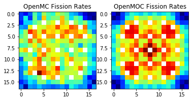
Flux and Pin Power Visualizations
We will conclude this tutorial by illustrating how to visualize the fission rates computed by OpenMOC and OpenMC. First, we extract volume-integrated fission rates from OpenMC’s mesh fission rate tally for each pin cell in the fuel assembly.
[38]:
# Get the OpenMC fission rate mesh tally data
mesh_tally = sp.get_tally(name='mesh tally')
openmc_fission_rates = mesh_tally.get_values(scores=['nu-fission'])

# Reshape array to 2D for plotting
openmc_fission_rates.shape = (17,17)

# Normalize to the average pin power
openmc_fission_rates /= np.mean(openmc_fission_rates[openmc_fission_rates > 0.])
Next, we extract OpenMOC’s volume-averaged fission rates into a 2D 17x17 NumPy array.
[39]:
# Create OpenMOC Mesh on which to tally fission rates
openmoc_mesh = openmoc.process.Mesh()
openmoc_mesh.dimension = np.array(mesh.dimension)
openmoc_mesh.lower_left = np.array(mesh.lower_left)
openmoc_mesh.upper_right = np.array(mesh.upper_right)
openmoc_mesh.width = openmoc_mesh.upper_right - openmoc_mesh.lower_left
openmoc_mesh.width /= openmoc_mesh.dimension

# Tally OpenMOC fission rates on the Mesh
openmoc_fission_rates = openmoc_mesh.tally_fission_rates(solver)
openmoc_fission_rates = np.squeeze(openmoc_fission_rates)
openmoc_fission_rates = np.fliplr(openmoc_fission_rates)

# Normalize to the average pin fission rate
openmoc_fission_rates /= np.mean(openmoc_fission_rates[openmoc_fission_rates > 0.])
Now we can easily use Matplotlib to visualize the fission rates from OpenMC and OpenMOC side-by-side.
[40]:
# Ignore zero fission rates in guide tubes with Matplotlib color scheme
openmc_fission_rates[openmc_fission_rates == 0] = np.nan
openmoc_fission_rates[openmoc_fission_rates == 0] = np.nan

# Plot OpenMC's fission rates in the left subplot
fig = plt.subplot(121)
plt.imshow(openmc_fission_rates, interpolation='none', cmap='jet')
plt.title('OpenMC Fission Rates')

# Plot OpenMOC's fission rates in the right subplot
fig2 = plt.subplot(122)
plt.imshow(openmoc_fission_rates, interpolation='none', cmap='jet')
plt.title('OpenMOC Fission Rates')
[40]:
Text(0.5, 1.0, 'OpenMOC Fission Rates')