Multigroup (Delayed) Cross Section Generation Part II: Advanced Features
This IPython Notebook illustrates the use of the ``openmc.mgxs.Library`` class. The Library class is designed to automate the calculation of multi-group cross sections for use cases with one or more domains, cross section types, and/or nuclides. In particular, this Notebook illustrates the following features:
- Calculation of multi-energy-group and multi-delayed-group cross sections for a fuel assembly
- Automated creation, manipulation and storage of
MGXSwith ``openmc.mgxs.Library`` - Steady-state pin-by-pin delayed neutron fractions (beta) for each delayed group.
- Generation of surface currents on the interfaces and surfaces of a Mesh.
Generate Input Files
[1]:
%matplotlib inline
import math

import matplotlib.pyplot as plt
import numpy as np

import openmc
import openmc.mgxs
First we need to define materials that will be used in the problem: fuel, water, and cladding.
[2]:
# 1.6 enriched fuel
fuel = openmc.Material(name='1.6% Fuel')
fuel.set_density('g/cm3', 10.31341)
fuel.add_nuclide('U235', 3.7503e-4)
fuel.add_nuclide('U238', 2.2625e-2)
fuel.add_nuclide('O16', 4.6007e-2)

# borated water
water = openmc.Material(name='Borated Water')
water.set_density('g/cm3', 0.740582)
water.add_nuclide('H1', 4.9457e-2)
water.add_nuclide('O16', 2.4732e-2)
water.add_nuclide('B10', 8.0042e-6)

# zircaloy
zircaloy = openmc.Material(name='Zircaloy')
zircaloy.set_density('g/cm3', 6.55)
zircaloy.add_nuclide('Zr90', 7.2758e-3)
With our three materials, we can now create a Materials object that can be exported to an actual XML file.
[3]:
# Create a materials collection and export to XML
materials = openmc.Materials((fuel, water, zircaloy))
materials.export_to_xml()
Now let’s move on to the geometry. This problem will be a square array of fuel pins and control rod guide tubes for which we can use OpenMC’s lattice/universe feature. The basic universe will have three regions for the fuel, the clad, and the surrounding coolant. The first step is to create the bounding surfaces for fuel and clad, as well as the outer bounding surfaces of the problem.
[4]:
# Create cylinders for the fuel and clad
fuel_outer_radius = openmc.ZCylinder(r=0.39218)
clad_outer_radius = openmc.ZCylinder(r=0.45720)

# Create boundary planes to surround the geometry
min_x = openmc.XPlane(x0=-10.71, boundary_type='reflective')
max_x = openmc.XPlane(x0=+10.71, boundary_type='reflective')
min_y = openmc.YPlane(y0=-10.71, boundary_type='reflective')
max_y = openmc.YPlane(y0=+10.71, boundary_type='reflective')
min_z = openmc.ZPlane(z0=-10., boundary_type='reflective')
max_z = openmc.ZPlane(z0=+10., boundary_type='reflective')
With the surfaces defined, we can now construct a fuel pin cell from cells that are defined by intersections of half-spaces created by the surfaces.
[5]:
# Create a Universe to encapsulate a fuel pin
fuel_pin_universe = openmc.Universe(name='1.6% Fuel Pin')

# Create fuel Cell
fuel_cell = openmc.Cell(name='1.6% Fuel')
fuel_cell.fill = fuel
fuel_cell.region = -fuel_outer_radius
fuel_pin_universe.add_cell(fuel_cell)

# Create a clad Cell
clad_cell = openmc.Cell(name='1.6% Clad')
clad_cell.fill = zircaloy
clad_cell.region = +fuel_outer_radius & -clad_outer_radius
fuel_pin_universe.add_cell(clad_cell)

# Create a moderator Cell
moderator_cell = openmc.Cell(name='1.6% Moderator')
moderator_cell.fill = water
moderator_cell.region = +clad_outer_radius
fuel_pin_universe.add_cell(moderator_cell)
Likewise, we can construct a control rod guide tube with the same surfaces.
[6]:
# Create a Universe to encapsulate a control rod guide tube
guide_tube_universe = openmc.Universe(name='Guide Tube')

# Create guide tube Cell
guide_tube_cell = openmc.Cell(name='Guide Tube Water')
guide_tube_cell.fill = water
guide_tube_cell.region = -fuel_outer_radius
guide_tube_universe.add_cell(guide_tube_cell)

# Create a clad Cell
clad_cell = openmc.Cell(name='Guide Clad')
clad_cell.fill = zircaloy
clad_cell.region = +fuel_outer_radius & -clad_outer_radius
guide_tube_universe.add_cell(clad_cell)

# Create a moderator Cell
moderator_cell = openmc.Cell(name='Guide Tube Moderator')
moderator_cell.fill = water
moderator_cell.region = +clad_outer_radius
guide_tube_universe.add_cell(moderator_cell)
Using the pin cell universe, we can construct a 17x17 rectangular lattice with a 1.26 cm pitch.
[7]:
# Create fuel assembly Lattice
assembly = openmc.RectLattice(name='1.6% Fuel Assembly')
assembly.pitch = (1.26, 1.26)
assembly.lower_left = [-1.26 * 17. / 2.0] * 2
Next, we create a NumPy array of fuel pin and guide tube universes for the lattice.
[8]:
# Create array indices for guide tube locations in lattice
template_x = np.array([5, 8, 11, 3, 13, 2, 5, 8, 11, 14, 2, 5, 8,
                       11, 14, 2, 5, 8, 11, 14, 3, 13, 5, 8, 11])
template_y = np.array([2, 2, 2, 3, 3, 5, 5, 5, 5, 5, 8, 8, 8, 8,
                       8, 11, 11, 11, 11, 11, 13, 13, 14, 14, 14])

# Create universes array with the fuel pin and guide tube universes
universes = np.tile(fuel_pin_universe, (17,17))
universes[template_x, template_y] = guide_tube_universe

# Store the array of universes in the lattice
assembly.universes = universes
OpenMC requires that there is a “root” universe. Let us create a root cell that is filled by the pin cell universe and then assign it to the root universe.
[9]:
# Create root Cell
root_cell = openmc.Cell(name='root cell', fill=assembly)

# Add boundary planes
root_cell.region = +min_x & -max_x & +min_y & -max_y & +min_z & -max_z

# Create root Universe
root_universe = openmc.Universe(universe_id=0, name='root universe')
root_universe.add_cell(root_cell)
We now must create a geometry that is assigned a root universe and export it to XML.
[10]:
# Create Geometry and export to XML
geometry = openmc.Geometry(root_universe)
geometry.export_to_xml()
With the geometry and materials finished, we now just need to define simulation parameters. In this case, we will use 10 inactive batches and 40 active batches each with 2500 particles.
[11]:
# OpenMC simulation parameters
batches = 50
inactive = 10
particles = 2500

# Instantiate a Settings object
settings = openmc.Settings()
settings.batches = batches
settings.inactive = inactive
settings.particles = particles
settings.output = {'tallies': False}

# Create an initial uniform spatial source distribution over fissionable zones
bounds = [-10.71, -10.71, -10, 10.71, 10.71, 10.]
uniform_dist = openmc.stats.Box(bounds[:3], bounds[3:], only_fissionable=True)
settings.source = openmc.Source(space=uniform_dist)

# Export to "settings.xml"
settings.export_to_xml()
Let us also create a plot to verify that our fuel assembly geometry was created successfully.
[12]:
# Plot our geometry
plot = openmc.Plot.from_geometry(geometry)
plot.pixels = (250, 250)
plot.color_by = 'material'
openmc.plot_inline(plot)

As we can see from the plot, we have a nice array of fuel and guide tube pin cells with fuel, cladding, and water!
Create an MGXS Library
Now we are ready to generate multi-group cross sections! First, let’s define a 20-energy-group and 1-energy-group.
[13]:
# Instantiate a 20-group EnergyGroups object
energy_groups = openmc.mgxs.EnergyGroups()
energy_groups.group_edges = np.logspace(-3, 7.3, 21)

# Instantiate a 1-group EnergyGroups object
one_group = openmc.mgxs.EnergyGroups()
one_group.group_edges = np.array([energy_groups.group_edges[0], energy_groups.group_edges[-1]])
Next, we will instantiate an openmc.mgxs.Library for the energy and delayed groups with our the fuel assembly geometry.
[14]:
# Instantiate a tally mesh
mesh = openmc.RegularMesh(mesh_id=1)
mesh.dimension = [17, 17, 1]
mesh.lower_left = [-10.71, -10.71, -10000.]
mesh.width = [1.26, 1.26, 20000.]

# Initialize an 20-energy-group and 6-delayed-group MGXS Library
mgxs_lib = openmc.mgxs.Library(geometry)
mgxs_lib.energy_groups  = energy_groups
mgxs_lib.num_delayed_groups = 6

# Specify multi-group cross section types to compute
mgxs_lib.mgxs_types = ['total', 'transport', 'nu-scatter matrix', 'kappa-fission', 'inverse-velocity', 'chi-prompt',
                      'prompt-nu-fission', 'chi-delayed', 'delayed-nu-fission', 'beta']

# Specify a "mesh" domain type for the cross section tally filters
mgxs_lib.domain_type = 'mesh'

# Specify the mesh domain over which to compute multi-group cross sections
mgxs_lib.domains = [mesh]

# Construct all tallies needed for the multi-group cross section library
mgxs_lib.build_library()

# Create a "tallies.xml" file for the MGXS Library
tallies_file = openmc.Tallies()
mgxs_lib.add_to_tallies_file(tallies_file, merge=True)

# Instantiate a current tally
mesh_filter = openmc.MeshSurfaceFilter(mesh)
current_tally = openmc.Tally(name='current tally')
current_tally.scores = ['current']
current_tally.filters = [mesh_filter]

# Add current tally to the tallies file
tallies_file.append(current_tally)

# Export to "tallies.xml"
tallies_file.export_to_xml()
/home/romano/openmc/openmc/mixin.py:71: IDWarning: Another Filter instance already exists with id=1.
  warn(msg, IDWarning)
/home/romano/openmc/openmc/mixin.py:71: IDWarning: Another Filter instance already exists with id=2.
  warn(msg, IDWarning)
/home/romano/openmc/openmc/mixin.py:71: IDWarning: Another Filter instance already exists with id=5.
  warn(msg, IDWarning)
/home/romano/openmc/openmc/mixin.py:71: IDWarning: Another Filter instance already exists with id=6.
  warn(msg, IDWarning)
/home/romano/openmc/openmc/mixin.py:71: IDWarning: Another Filter instance already exists with id=17.
  warn(msg, IDWarning)
/home/romano/openmc/openmc/mixin.py:71: IDWarning: Another Filter instance already exists with id=23.
  warn(msg, IDWarning)
Now, we can run OpenMC to generate the cross sections.
[15]:
# Run OpenMC
openmc.run()
                                %%%%%%%%%%%%%%%
                           %%%%%%%%%%%%%%%%%%%%%%%%
                        %%%%%%%%%%%%%%%%%%%%%%%%%%%%%%
                      %%%%%%%%%%%%%%%%%%%%%%%%%%%%%%%%%%
                    %%%%%%%%%%%%%%%%%%%%%%%%%%%%%%%%%%%%%%
                   %%%%%%%%%%%%%%%%%%%%%%%%%%%%%%%%%%%%%%%%
                                    %%%%%%%%%%%%%%%%%%%%%%%%
                                     %%%%%%%%%%%%%%%%%%%%%%%%
                 ###############      %%%%%%%%%%%%%%%%%%%%%%%%
                ##################     %%%%%%%%%%%%%%%%%%%%%%%
                ###################     %%%%%%%%%%%%%%%%%%%%%%%
                ####################     %%%%%%%%%%%%%%%%%%%%%%
                #####################     %%%%%%%%%%%%%%%%%%%%%
                ######################     %%%%%%%%%%%%%%%%%%%%
                #######################     %%%%%%%%%%%%%%%%%%
                 #######################     %%%%%%%%%%%%%%%%%
                 ######################     %%%%%%%%%%%%%%%%%
                  ####################     %%%%%%%%%%%%%%%%%
                    #################     %%%%%%%%%%%%%%%%%
                     ###############     %%%%%%%%%%%%%%%%
                       ############     %%%%%%%%%%%%%%%
                          ########     %%%%%%%%%%%%%%
                                      %%%%%%%%%%%

                   | The OpenMC Monte Carlo Code
         Copyright | 2011-2019 MIT and OpenMC contributors
           License | http://openmc.readthedocs.io/en/latest/license.html
           Version | 0.11.0-dev
          Git SHA1 | 61c911cffdae2406f9f4bc667a9a6954748bb70c
         Date/Time | 2019-07-18 22:07:58
    OpenMP Threads | 4

 Reading settings XML file...
 Reading cross sections XML file...
 Reading materials XML file...
 Reading geometry XML file...
 Reading U235 from /opt/data/hdf5/nndc_hdf5_v15/U235.h5
 Reading U238 from /opt/data/hdf5/nndc_hdf5_v15/U238.h5
 Reading O16 from /opt/data/hdf5/nndc_hdf5_v15/O16.h5
 Reading H1 from /opt/data/hdf5/nndc_hdf5_v15/H1.h5
 Reading B10 from /opt/data/hdf5/nndc_hdf5_v15/B10.h5
 Reading Zr90 from /opt/data/hdf5/nndc_hdf5_v15/Zr90.h5
 Maximum neutron transport energy: 20000000.000000 eV for U235
 Reading tallies XML file...
 Writing summary.h5 file...
 Initializing source particles...

 ====================>     K EIGENVALUE SIMULATION     <====================

  Bat./Gen.      k            Average k
  =========   ========   ====================
        1/1    1.03852
        2/1    0.99743
        3/1    1.02987
        4/1    1.04397
        5/1    1.06262
        6/1    1.06657
        7/1    0.98574
        8/1    1.04364
        9/1    1.01253
       10/1    1.02094
       11/1    0.99586
       12/1    1.00508    1.00047 +/- 0.00461
       13/1    1.05292    1.01795 +/- 0.01769
       14/1    1.04732    1.02530 +/- 0.01450
       15/1    1.04886    1.03001 +/- 0.01218
       16/1    1.00948    1.02659 +/- 0.01052
       17/1    1.02644    1.02657 +/- 0.00889
       18/1    1.03080    1.02710 +/- 0.00772
       19/1    1.00018    1.02411 +/- 0.00743
       20/1    1.05668    1.02736 +/- 0.00740
       21/1    1.01160    1.02593 +/- 0.00685
       22/1    1.04334    1.02738 +/- 0.00642
       23/1    1.03105    1.02766 +/- 0.00591
       24/1    1.01174    1.02653 +/- 0.00559
       25/1    0.99844    1.02465 +/- 0.00553
       26/1    1.02241    1.02451 +/- 0.00517
       27/1    1.02904    1.02478 +/- 0.00487
       28/1    1.02132    1.02459 +/- 0.00459
       29/1    1.01384    1.02402 +/- 0.00438
       30/1    1.03891    1.02477 +/- 0.00422
       31/1    1.04092    1.02553 +/- 0.00409
       32/1    1.00058    1.02440 +/- 0.00406
       33/1    0.99940    1.02331 +/- 0.00403
       34/1    0.98362    1.02166 +/- 0.00420
       35/1    1.05358    1.02294 +/- 0.00422
       36/1    0.99923    1.02202 +/- 0.00416
       37/1    1.08491    1.02435 +/- 0.00463
       38/1    1.01838    1.02414 +/- 0.00447
       39/1    0.98567    1.02281 +/- 0.00451
       40/1    1.05047    1.02374 +/- 0.00445
       41/1    1.01993    1.02361 +/- 0.00431
       42/1    1.01223    1.02326 +/- 0.00419
       43/1    1.06259    1.02445 +/- 0.00423
       44/1    1.01993    1.02432 +/- 0.00411
       45/1    0.99233    1.02340 +/- 0.00409
       46/1    0.98532    1.02234 +/- 0.00411
       47/1    1.02513    1.02242 +/- 0.00400
       48/1    1.01637    1.02226 +/- 0.00390
       49/1    1.03215    1.02251 +/- 0.00381
       50/1    1.01826    1.02241 +/- 0.00371
 Creating state point statepoint.50.h5...

 =======================>     TIMING STATISTICS     <=======================

 Total time for initialization     = 4.2397e-01 seconds
   Reading cross sections          = 4.0321e-01 seconds
 Total time in simulation          = 2.0407e+01 seconds
   Time in transport only          = 2.0154e+01 seconds
   Time in inactive batches        = 1.0937e+00 seconds
   Time in active batches          = 1.9314e+01 seconds
   Time synchronizing fission bank = 7.8056e-03 seconds
     Sampling source sites         = 6.7223e-03 seconds
     SEND/RECV source sites        = 9.5783e-04 seconds
   Time accumulating tallies       = 9.2006e-02 seconds
 Total time for finalization       = 1.0890e-02 seconds
 Total time elapsed                = 2.0869e+01 seconds
 Calculation Rate (inactive)       = 22858.4 particles/second
 Calculation Rate (active)         = 5177.70 particles/second

 ============================>     RESULTS     <============================

 k-effective (Collision)     = 1.02207 +/- 0.00343
 k-effective (Track-length)  = 1.02241 +/- 0.00371
 k-effective (Absorption)    = 1.02408 +/- 0.00356
 Combined k-effective        = 1.02306 +/- 0.00307
 Leakage Fraction            = 0.00000 +/- 0.00000
Tally Data Processing
Our simulation ran successfully and created statepoint and summary output files. We begin our analysis by instantiating a StatePoint object.
[16]:
# Load the last statepoint file
sp = openmc.StatePoint('statepoint.50.h5')
The statepoint is now ready to be analyzed by the Library. We simply have to load the tallies from the statepoint into the Library and our MGXS objects will compute the cross sections for us under-the-hood.
[17]:
# Initialize MGXS Library with OpenMC statepoint data
mgxs_lib.load_from_statepoint(sp)

# Extrack the current tally separately
current_tally = sp.get_tally(name='current tally')
Using Tally Arithmetic to Compute the Delayed Neutron Precursor Concentrations
Finally, we illustrate how one can leverage OpenMC’s tally arithmetic data processing feature with MGXS objects. The openmc.mgxs module uses tally arithmetic to compute multi-group cross sections with automated uncertainty propagation. Each MGXS object includes an xs_tally attribute which is a “derived” Tally based on the tallies needed to compute the cross section type of interest. These derived tallies can be used in subsequent tally arithmetic
operations. For example, we can use tally artithmetic to compute the delayed neutron precursor concentrations using the Beta and DelayedNuFissionXS objects. The delayed neutron precursor concentrations are modeled using the following equations:
[18]:
# Set the time constants for the delayed precursors (in seconds^-1)
precursor_halflife = np.array([55.6, 24.5, 16.3, 2.37, 0.424, 0.195])
precursor_lambda = math.log(2.0) / precursor_halflife

beta = mgxs_lib.get_mgxs(mesh, 'beta')

# Create a tally object with only the delayed group filter for the time constants
beta_filters = [f for f in beta.xs_tally.filters if type(f) is not openmc.DelayedGroupFilter]
lambda_tally = beta.xs_tally.summation(nuclides=beta.xs_tally.nuclides)
for f in beta_filters:
    lambda_tally = lambda_tally.summation(filter_type=type(f), remove_filter=True) * 0. + 1.

# Set the mean of the lambda tally and reshape to account for nuclides and scores
lambda_tally._mean = precursor_lambda
lambda_tally._mean.shape = lambda_tally.std_dev.shape

# Set a total nuclide and lambda score
lambda_tally.nuclides = [openmc.Nuclide(name='total')]
lambda_tally.scores = ['lambda']

delayed_nu_fission = mgxs_lib.get_mgxs(mesh, 'delayed-nu-fission')

# Use tally arithmetic to compute the precursor concentrations
precursor_conc = beta.xs_tally.summation(filter_type=openmc.EnergyFilter, remove_filter=True) * \
    delayed_nu_fission.xs_tally.summation(filter_type=openmc.EnergyFilter, remove_filter=True) / lambda_tally

# The difference is a derived tally which can generate Pandas DataFrames for inspection
precursor_conc.get_pandas_dataframe().head(10)
[18]:
| mesh 1 | delayedgroup | nuclide | score | mean | std. dev. | |||
|---|---|---|---|---|---|---|---|---|
| x | y | z | ||||||
| 0 | 1 | 1 | 1 | 1 | total | (((delayed-nu-fission / nu-fission) * (delayed... | 0.000099 | 2.275247e-05 |
| 1 | 1 | 1 | 1 | 2 | total | (((delayed-nu-fission / nu-fission) * (delayed... | 0.001260 | 2.852271e-04 |
| 2 | 1 | 1 | 1 | 3 | total | (((delayed-nu-fission / nu-fission) * (delayed... | 0.000800 | 1.795615e-04 |
| 3 | 1 | 1 | 1 | 4 | total | (((delayed-nu-fission / nu-fission) * (delayed... | 0.000630 | 1.397151e-04 |
| 4 | 1 | 1 | 1 | 5 | total | (((delayed-nu-fission / nu-fission) * (delayed... | 0.000023 | 4.861639e-06 |
| 5 | 1 | 1 | 1 | 6 | total | (((delayed-nu-fission / nu-fission) * (delayed... | 0.000002 | 3.879558e-07 |
| 6 | 2 | 1 | 1 | 1 | total | (((delayed-nu-fission / nu-fission) * (delayed... | 0.000091 | 2.062544e-05 |
| 7 | 2 | 1 | 1 | 2 | total | (((delayed-nu-fission / nu-fission) * (delayed... | 0.001162 | 2.584797e-04 |
| 8 | 2 | 1 | 1 | 3 | total | (((delayed-nu-fission / nu-fission) * (delayed... | 0.000737 | 1.626991e-04 |
| 9 | 2 | 1 | 1 | 4 | total | (((delayed-nu-fission / nu-fission) * (delayed... | 0.000581 | 1.265708e-04 |
Another useful feature of the Python API is the ability to extract the surface currents for the interfaces and surfaces of a mesh. We can inspect the currents for the mesh by getting the pandas dataframe.
[19]:
current_tally.get_pandas_dataframe().head(10)
[19]:
| mesh 1 | nuclide | score | mean | std. dev. | ||||
|---|---|---|---|---|---|---|---|---|
| x | y | z | surf | |||||
| 0 | 1 | 1 | 1 | x-min out | total | current | 0.00000 | 0.000000 |
| 1 | 1 | 1 | 1 | x-min in | total | current | 0.00000 | 0.000000 |
| 2 | 1 | 1 | 1 | x-max out | total | current | 0.03245 | 0.000677 |
| 3 | 1 | 1 | 1 | x-max in | total | current | 0.03180 | 0.000659 |
| 4 | 1 | 1 | 1 | y-min out | total | current | 0.00000 | 0.000000 |
| 5 | 1 | 1 | 1 | y-min in | total | current | 0.00000 | 0.000000 |
| 6 | 1 | 1 | 1 | y-max out | total | current | 0.03072 | 0.000677 |
| 7 | 1 | 1 | 1 | y-max in | total | current | 0.03104 | 0.000652 |
| 8 | 1 | 1 | 1 | z-min out | total | current | 0.00000 | 0.000000 |
| 9 | 1 | 1 | 1 | z-min in | total | current | 0.00000 | 0.000000 |
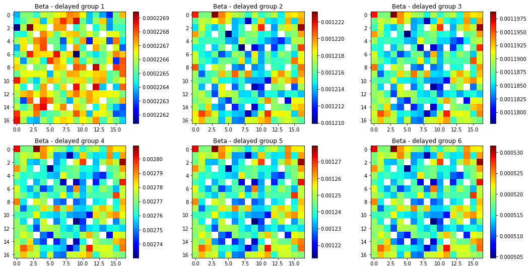
Cross Section Visualizations
In addition to inspecting the data in the tallies by getting the pandas dataframe, we can also plot the tally data on the domain mesh. Below is the delayed neutron fraction tallied in each mesh cell for each delayed group.
[20]:
# Extract the energy-condensed delayed neutron fraction tally
beta_by_group = beta.get_condensed_xs(one_group).xs_tally.summation(filter_type='energy', remove_filter=True)
beta_by_group.mean.shape = (17, 17, 6)
beta_by_group.mean[beta_by_group.mean == 0] = np.nan

# Plot the betas
plt.figure(figsize=(18,9))
fig = plt.subplot(231)
plt.imshow(beta_by_group.mean[:,:,0], interpolation='none', cmap='jet')
plt.colorbar()
plt.title('Beta - delayed group 1')

fig = plt.subplot(232)
plt.imshow(beta_by_group.mean[:,:,1], interpolation='none', cmap='jet')
plt.colorbar()
plt.title('Beta - delayed group 2')

fig = plt.subplot(233)
plt.imshow(beta_by_group.mean[:,:,2], interpolation='none', cmap='jet')
plt.colorbar()
plt.title('Beta - delayed group 3')

fig = plt.subplot(234)
plt.imshow(beta_by_group.mean[:,:,3], interpolation='none', cmap='jet')
plt.colorbar()
plt.title('Beta - delayed group 4')

fig = plt.subplot(235)
plt.imshow(beta_by_group.mean[:,:,4], interpolation='none', cmap='jet')
plt.colorbar()
plt.title('Beta - delayed group 5')

fig = plt.subplot(236)
plt.imshow(beta_by_group.mean[:,:,5], interpolation='none', cmap='jet')
plt.colorbar()
plt.title('Beta - delayed group 6')
[20]:
Text(0.5, 1.0, 'Beta - delayed group 6')