Post Processing
This notebook demonstrates some basic post-processing tasks that can be performed with the Python API, such as plotting a 2D mesh tally and plotting neutron source sites from an eigenvalue calculation. The problem we will use is a simple reflected pin-cell.
[1]:
%matplotlib inline
from IPython.display import Image
import numpy as np
import matplotlib.pyplot as plt
import openmc
Generate Input Files
First we need to define materials that will be used in the problem. We’ll create three materials for the fuel, water, and cladding of the fuel pin.
[2]:
# 1.6 enriched fuel
fuel = openmc.Material(name='1.6% Fuel')
fuel.set_density('g/cm3', 10.31341)
fuel.add_nuclide('U235', 3.7503e-4)
fuel.add_nuclide('U238', 2.2625e-2)
fuel.add_nuclide('O16', 4.6007e-2)

# borated water
water = openmc.Material(name='Borated Water')
water.set_density('g/cm3', 0.740582)
water.add_nuclide('H1', 4.9457e-2)
water.add_nuclide('O16', 2.4732e-2)
water.add_nuclide('B10', 8.0042e-6)

# zircaloy
zircaloy = openmc.Material(name='Zircaloy')
zircaloy.set_density('g/cm3', 6.55)
zircaloy.add_nuclide('Zr90', 7.2758e-3)
With our three materials, we can now create a materials file object that can be exported to an actual XML file.
[3]:
# Instantiate a Materials collection
materials = openmc.Materials([fuel, water, zircaloy])

# Export to "materials.xml"
materials.export_to_xml()
Now let’s move on to the geometry. Our problem will have three regions for the fuel, the clad, and the surrounding coolant. The first step is to create the bounding surfaces – in this case two cylinders and six reflective planes.
[4]:
# Create cylinders for the fuel and clad
fuel_outer_radius = openmc.ZCylinder(x0=0.0, y0=0.0, r=0.39218)
clad_outer_radius = openmc.ZCylinder(x0=0.0, y0=0.0, r=0.45720)

# Create boundary planes to surround the geometry
min_x = openmc.XPlane(x0=-0.63, boundary_type='reflective')
max_x = openmc.XPlane(x0=+0.63, boundary_type='reflective')
min_y = openmc.YPlane(y0=-0.63, boundary_type='reflective')
max_y = openmc.YPlane(y0=+0.63, boundary_type='reflective')
min_z = openmc.ZPlane(z0=-0.63, boundary_type='reflective')
max_z = openmc.ZPlane(z0=+0.63, boundary_type='reflective')
With the surfaces defined, we can now create cells that are defined by intersections of half-spaces created by the surfaces.
[5]:
# Create a Universe to encapsulate a fuel pin
pin_cell_universe = openmc.Universe(name='1.6% Fuel Pin')

# Create fuel Cell
fuel_cell = openmc.Cell(name='1.6% Fuel')
fuel_cell.fill = fuel
fuel_cell.region = -fuel_outer_radius
pin_cell_universe.add_cell(fuel_cell)

# Create a clad Cell
clad_cell = openmc.Cell(name='1.6% Clad')
clad_cell.fill = zircaloy
clad_cell.region = +fuel_outer_radius & -clad_outer_radius
pin_cell_universe.add_cell(clad_cell)

# Create a moderator Cell
moderator_cell = openmc.Cell(name='1.6% Moderator')
moderator_cell.fill = water
moderator_cell.region = +clad_outer_radius
pin_cell_universe.add_cell(moderator_cell)
OpenMC requires that there is a “root” universe. Let us create a root cell that is filled by the pin cell universe and then assign it to the root universe.
[6]:
# Create root Cell
root_cell = openmc.Cell(name='root cell')
root_cell.fill = pin_cell_universe

# Add boundary planes
root_cell.region = +min_x & -max_x & +min_y & -max_y & +min_z & -max_z

# Create root Universe
root_universe = openmc.Universe(universe_id=0, name='root universe')
root_universe.add_cell(root_cell)
We now must create a geometry that is assigned a root universe, put the geometry into a geometry file, and export it to XML.
[7]:
# Create Geometry and set root Universe
geometry = openmc.Geometry(root_universe)
[8]:
# Export to "geometry.xml"
geometry.export_to_xml()
With the geometry and materials finished, we now just need to define simulation parameters. In this case, we will use 10 inactive batches and 90 active batches each with 5000 particles.
[9]:
# OpenMC simulation parameters
settings = openmc.Settings()
settings.batches = 100
settings.inactive = 10
settings.particles = 5000

# Create an initial uniform spatial source distribution over fissionable zones
bounds = [-0.63, -0.63, -0.63, 0.63, 0.63, 0.63]
uniform_dist = openmc.stats.Box(bounds[:3], bounds[3:], only_fissionable=True)
settings.source = openmc.Source(space=uniform_dist)

# Export to "settings.xml"
settings.export_to_xml()
Let us also create a plot file that we can use to verify that our pin cell geometry was created successfully.
[10]:
plot = openmc.Plot.from_geometry(geometry)
plot.pixels = (250, 250)
plot.to_ipython_image()
[10]:

As we can see from the plot, we have a nice pin cell with fuel, cladding, and water! Before we run our simulation, we need to tell the code what we want to tally. The following code shows how to create a 2D mesh tally.
[11]:
# Instantiate an empty Tallies object
tallies = openmc.Tallies()
[12]:
# Create mesh which will be used for tally
mesh = openmc.RegularMesh()
mesh.dimension = [100, 100]
mesh.lower_left = [-0.63, -0.63]
mesh.upper_right = [0.63, 0.63]

# Create mesh filter for tally
mesh_filter = openmc.MeshFilter(mesh)

# Create mesh tally to score flux and fission rate
tally = openmc.Tally(name='flux')
tally.filters = [mesh_filter]
tally.scores = ['flux', 'fission']
tallies.append(tally)
[13]:
# Export to "tallies.xml"
tallies.export_to_xml()
Now we a have a complete set of inputs, so we can go ahead and run our simulation.
[14]:
# Run OpenMC!
openmc.run()
                                %%%%%%%%%%%%%%%
                           %%%%%%%%%%%%%%%%%%%%%%%%
                        %%%%%%%%%%%%%%%%%%%%%%%%%%%%%%
                      %%%%%%%%%%%%%%%%%%%%%%%%%%%%%%%%%%
                    %%%%%%%%%%%%%%%%%%%%%%%%%%%%%%%%%%%%%%
                   %%%%%%%%%%%%%%%%%%%%%%%%%%%%%%%%%%%%%%%%
                                    %%%%%%%%%%%%%%%%%%%%%%%%
                                     %%%%%%%%%%%%%%%%%%%%%%%%
                 ###############      %%%%%%%%%%%%%%%%%%%%%%%%
                ##################     %%%%%%%%%%%%%%%%%%%%%%%
                ###################     %%%%%%%%%%%%%%%%%%%%%%%
                ####################     %%%%%%%%%%%%%%%%%%%%%%
                #####################     %%%%%%%%%%%%%%%%%%%%%
                ######################     %%%%%%%%%%%%%%%%%%%%
                #######################     %%%%%%%%%%%%%%%%%%
                 #######################     %%%%%%%%%%%%%%%%%
                 ######################     %%%%%%%%%%%%%%%%%
                  ####################     %%%%%%%%%%%%%%%%%
                    #################     %%%%%%%%%%%%%%%%%
                     ###############     %%%%%%%%%%%%%%%%
                       ############     %%%%%%%%%%%%%%%
                          ########     %%%%%%%%%%%%%%
                                      %%%%%%%%%%%

                   | The OpenMC Monte Carlo Code
         Copyright | 2011-2019 MIT and OpenMC contributors
           License | http://openmc.readthedocs.io/en/latest/license.html
           Version | 0.11.0-dev
          Git SHA1 | 61c911cffdae2406f9f4bc667a9a6954748bb70c
         Date/Time | 2019-07-19 06:22:24
    OpenMP Threads | 4

 Reading settings XML file...
 Reading cross sections XML file...
 Reading materials XML file...
 Reading geometry XML file...
 Reading U235 from /opt/data/hdf5/nndc_hdf5_v15/U235.h5
 Reading U238 from /opt/data/hdf5/nndc_hdf5_v15/U238.h5
 Reading O16 from /opt/data/hdf5/nndc_hdf5_v15/O16.h5
 Reading H1 from /opt/data/hdf5/nndc_hdf5_v15/H1.h5
 Reading B10 from /opt/data/hdf5/nndc_hdf5_v15/B10.h5
 Reading Zr90 from /opt/data/hdf5/nndc_hdf5_v15/Zr90.h5
 Maximum neutron transport energy: 20000000.000000 eV for U235
 Reading tallies XML file...
 Writing summary.h5 file...
 Initializing source particles...

 ====================>     K EIGENVALUE SIMULATION     <====================

  Bat./Gen.      k            Average k
  =========   ========   ====================
        1/1    1.04359
        2/1    1.04323
        3/1    1.04711
        4/1    1.03892
        5/1    1.02459
        6/1    1.03936
        7/1    1.03529
        8/1    1.01590
        9/1    1.03060
       10/1    1.02892
       11/1    1.03987
       12/1    1.04395    1.04191 +/- 0.00204
       13/1    1.04971    1.04451 +/- 0.00285
       14/1    1.03880    1.04308 +/- 0.00247
       15/1    1.03091    1.04065 +/- 0.00310
       16/1    1.03618    1.03990 +/- 0.00264
       17/1    1.04109    1.04007 +/- 0.00223
       18/1    1.02978    1.03879 +/- 0.00232
       19/1    1.06363    1.04155 +/- 0.00344
       20/1    1.06549    1.04394 +/- 0.00390
       21/1    1.03469    1.04310 +/- 0.00362
       22/1    1.01925    1.04111 +/- 0.00386
       23/1    1.03268    1.04046 +/- 0.00361
       24/1    1.03906    1.04036 +/- 0.00334
       25/1    1.02632    1.03943 +/- 0.00325
       26/1    1.03906    1.03940 +/- 0.00304
       27/1    1.05058    1.04006 +/- 0.00293
       28/1    1.03248    1.03964 +/- 0.00279
       29/1    1.04076    1.03970 +/- 0.00264
       30/1    1.00994    1.03821 +/- 0.00292
       31/1    1.04785    1.03867 +/- 0.00281
       32/1    1.03080    1.03831 +/- 0.00270
       33/1    1.01862    1.03746 +/- 0.00272
       34/1    1.05370    1.03813 +/- 0.00269
       35/1    1.02226    1.03750 +/- 0.00266
       36/1    1.02862    1.03716 +/- 0.00258
       37/1    1.04790    1.03755 +/- 0.00251
       38/1    1.03762    1.03756 +/- 0.00242
       39/1    1.02255    1.03704 +/- 0.00239
       40/1    1.06094    1.03784 +/- 0.00245
       41/1    1.03842    1.03786 +/- 0.00237
       42/1    1.00628    1.03687 +/- 0.00249
       43/1    1.04916    1.03724 +/- 0.00245
       44/1    1.06237    1.03798 +/- 0.00248
       45/1    1.08153    1.03922 +/- 0.00271
       46/1    1.05649    1.03970 +/- 0.00268
       47/1    1.06265    1.04032 +/- 0.00268
       48/1    1.05728    1.04077 +/- 0.00265
       49/1    1.07343    1.04161 +/- 0.00271
       50/1    1.04640    1.04173 +/- 0.00265
       51/1    1.05143    1.04196 +/- 0.00259
       52/1    1.03639    1.04183 +/- 0.00253
       53/1    1.04846    1.04199 +/- 0.00248
       54/1    1.02435    1.04158 +/- 0.00245
       55/1    1.04806    1.04173 +/- 0.00240
       56/1    1.04798    1.04186 +/- 0.00235
       57/1    1.06621    1.04238 +/- 0.00236
       58/1    1.05734    1.04269 +/- 0.00233
       59/1    1.04581    1.04276 +/- 0.00228
       60/1    1.02682    1.04244 +/- 0.00226
       61/1    1.05971    1.04278 +/- 0.00224
       62/1    1.02357    1.04241 +/- 0.00223
       63/1    1.02645    1.04211 +/- 0.00221
       64/1    1.00711    1.04146 +/- 0.00226
       65/1    1.06171    1.04183 +/- 0.00225
       66/1    1.03444    1.04170 +/- 0.00221
       67/1    1.05875    1.04199 +/- 0.00219
       68/1    1.04640    1.04207 +/- 0.00216
       69/1    1.04376    1.04210 +/- 0.00212
       70/1    1.07078    1.04258 +/- 0.00214
       71/1    1.03916    1.04252 +/- 0.00210
       72/1    1.01843    1.04213 +/- 0.00211
       73/1    1.03666    1.04205 +/- 0.00207
       74/1    1.04625    1.04211 +/- 0.00204
       75/1    1.05277    1.04228 +/- 0.00202
       76/1    1.04944    1.04238 +/- 0.00199
       77/1    1.01898    1.04203 +/- 0.00199
       78/1    1.03283    1.04190 +/- 0.00197
       79/1    1.02304    1.04163 +/- 0.00196
       80/1    1.01539    1.04125 +/- 0.00196
       81/1    1.03988    1.04123 +/- 0.00194
       82/1    1.02138    1.04096 +/- 0.00193
       83/1    1.02473    1.04073 +/- 0.00192
       84/1    1.03810    1.04070 +/- 0.00189
       85/1    1.07438    1.04115 +/- 0.00192
       86/1    1.03048    1.04101 +/- 0.00190
       87/1    1.06778    1.04135 +/- 0.00191
       88/1    1.07341    1.04177 +/- 0.00192
       89/1    1.06729    1.04209 +/- 0.00193
       90/1    1.05069    1.04220 +/- 0.00191
       91/1    1.07675    1.04262 +/- 0.00193
       92/1    1.06470    1.04289 +/- 0.00193
       93/1    1.02609    1.04269 +/- 0.00191
       94/1    1.04761    1.04275 +/- 0.00189
       95/1    1.08802    1.04328 +/- 0.00194
       96/1    1.04162    1.04326 +/- 0.00192
       97/1    1.04573    1.04329 +/- 0.00190
       98/1    1.03232    1.04317 +/- 0.00188
       99/1    1.03473    1.04307 +/- 0.00186
      100/1    1.04505    1.04309 +/- 0.00184
 Creating state point statepoint.100.h5...

 =======================>     TIMING STATISTICS     <=======================

 Total time for initialization     = 6.4445e-01 seconds
   Reading cross sections          = 6.1129e-01 seconds
 Total time in simulation          = 2.0000e+02 seconds
   Time in transport only          = 1.9970e+02 seconds
   Time in inactive batches        = 2.9966e+00 seconds
   Time in active batches          = 1.9701e+02 seconds
   Time synchronizing fission bank = 4.0040e-02 seconds
     Sampling source sites         = 3.1522e-02 seconds
     SEND/RECV source sites        = 8.3459e-03 seconds
   Time accumulating tallies       = 9.3582e-03 seconds
 Total time for finalization       = 4.6582e-02 seconds
 Total time elapsed                = 2.0072e+02 seconds
 Calculation Rate (inactive)       = 16685.4 particles/second
 Calculation Rate (active)         = 2284.19 particles/second

 ============================>     RESULTS     <============================

 k-effective (Collision)     = 1.04342 +/- 0.00159
 k-effective (Track-length)  = 1.04309 +/- 0.00184
 k-effective (Absorption)    = 1.04107 +/- 0.00140
 Combined k-effective        = 1.04195 +/- 0.00117
 Leakage Fraction            = 0.00000 +/- 0.00000
Tally Data Processing
Our simulation ran successfully and created a statepoint file with all the tally data in it. We begin our analysis here loading the statepoint file and ‘reading’ the results. By default, data from the statepoint file is only read into memory when it is requested. This helps keep the memory use to a minimum even when a statepoint file may be huge.
[15]:
# Load the statepoint file
sp = openmc.StatePoint('statepoint.100.h5')
Next we need to get the tally, which can be done with the StatePoint.get_tally(...) method.
[16]:
tally = sp.get_tally(scores=['flux'])
print(tally)
Tally
        ID             =        1
        Name           =        flux
        Filters        =        MeshFilter
        Nuclides       =        total
        Scores         =        ['flux', 'fission']
        Estimator      =        tracklength
The statepoint file actually stores the sum and sum-of-squares for each tally bin from which the mean and variance can be calculated as described here. The sum and sum-of-squares can be accessed using the sum and sum_sq properties:
[17]:
tally.sum
[17]:
array([[[0.40767451, 0.        ]],

       [[0.40933814, 0.        ]],

       [[0.4119165 , 0.        ]],

       ...,

       [[0.40854327, 0.        ]],

       [[0.40970805, 0.        ]],

       [[0.40948065, 0.        ]]])
However, the mean and standard deviation of the mean are usually what you are more interested in. The Tally class also has properties mean and std_dev which automatically calculate these statistics on-the-fly.
[18]:
print(tally.mean.shape)
(tally.mean, tally.std_dev)
(10000, 1, 2)
[18]:
(array([[[0.00452972, 0.        ]],

        [[0.0045482 , 0.        ]],

        [[0.00457685, 0.        ]],

        ...,

        [[0.00453937, 0.        ]],

        [[0.00455231, 0.        ]],

        [[0.00454978, 0.        ]]]),
 array([[[2.03553236e-05, 0.00000000e+00]],

        [[1.83847389e-05, 0.00000000e+00]],

        [[1.68647098e-05, 0.00000000e+00]],

        ...,

        [[1.71606078e-05, 0.00000000e+00]],

        [[1.87645811e-05, 0.00000000e+00]],

        [[1.94447454e-05, 0.00000000e+00]]]))
The tally data has three dimensions: one for filter combinations, one for nuclides, and one for scores. We see that there are 10000 filter combinations (corresponding to the 100 x 100 mesh bins), a single nuclide (since none was specified), and two scores. If we only want to look at a single score, we can use the get_slice(...) method as follows.
[19]:
flux = tally.get_slice(scores=['flux'])
fission = tally.get_slice(scores=['fission'])
print(flux)
Tally
        ID             =        2
        Name           =        flux
        Filters        =        MeshFilter
        Nuclides       =        total
        Scores         =        ['flux']
        Estimator      =        tracklength
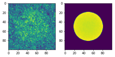
To get the bins into a form that we can plot, we can simply change the shape of the array since it is a numpy array.
[20]:
flux.std_dev.shape = (100, 100)
flux.mean.shape = (100, 100)
fission.std_dev.shape = (100, 100)
fission.mean.shape = (100, 100)
[21]:
fig = plt.subplot(121)
fig.imshow(flux.mean)
fig2 = plt.subplot(122)
fig2.imshow(fission.mean)
[21]:
<matplotlib.image.AxesImage at 0x14d12e58cb38>
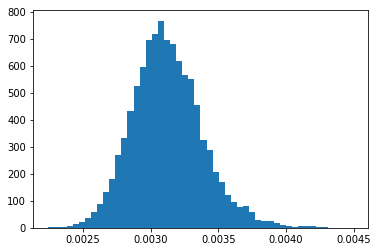
Now let’s say we want to look at the distribution of relative errors of our tally bins for flux. First we create a new variable called relative_error and set it to the ratio of the standard deviation and the mean, being careful not to divide by zero in case some bins were never scored to.
[22]:
# Determine relative error
relative_error = np.zeros_like(flux.std_dev)
nonzero = flux.mean > 0
relative_error[nonzero] = flux.std_dev[nonzero] / flux.mean[nonzero]

# distribution of relative errors
ret = plt.hist(relative_error[nonzero], bins=50)
Source Sites
Source sites can be accessed from the source property. As shown below, the source sites are represented as a numpy array with a structured datatype.
[23]:
sp.source
[23]:
array([((-0.28690552, -0.23731283,  0.51447853), ( 0.02705364, -0.14292142,  0.98936422), 1780128.70101981, 1., 0, 0),
       ((-0.28690552, -0.23731283,  0.51447853), (-0.16786951,  0.86432444, -0.47409186), 1553436.10501094, 1., 0, 0),
       (( 0.17162994,  0.134092  ,  0.42932363), ( 0.25199134, -0.11168216,  0.96126347),  829530.02360943, 1., 0, 0),
       ...,
       ((-0.24444068, -0.01351615, -0.41772172), ( 0.10437178, -0.86754673,  0.486281  ),  807617.55637656, 1., 0, 0),
       ((-0.2146841 ,  0.14307096,  0.07419328), ( 0.89645066, -0.35557279, -0.26446968), 6036005.44157462, 1., 0, 0),
       ((-0.2146841 ,  0.14307096,  0.07419328), (-0.95287644, -0.25857878,  0.15863005), 4923751.04163063, 1., 0, 0)],
      dtype=[('r', [('x', '<f8'), ('y', '<f8'), ('z', '<f8')]), ('u', [('x', '<f8'), ('y', '<f8'), ('z', '<f8')]), ('E', '<f8'), ('wgt', '<f8'), ('delayed_group', '<i4'), ('particle', '<i4')])
If we want, say, only the energies from the source sites, we can simply index the source array with the name of the field:
[24]:
sp.source['E']
[24]:
array([1780128.70101981, 1553436.10501094,  829530.02360943, ...,
        807617.55637656, 6036005.44157462, 4923751.04163063])
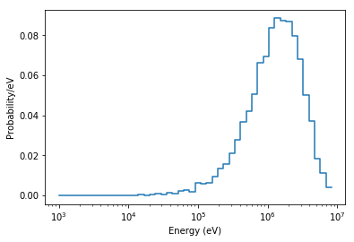
Now, we can look at things like the energy distribution of source sites. Note that we don’t directly use the matplotlib.pyplot.hist method since our binning is logarithmic.
[25]:
# Create log-spaced energy bins from 1 keV to 10 MeV
energy_bins = np.logspace(3,7)

# Calculate pdf for source energies
probability, bin_edges = np.histogram(sp.source['E'], energy_bins, density=True)

# Make sure integrating the PDF gives us unity
print(sum(probability*np.diff(energy_bins)))

# Plot source energy PDF
plt.semilogx(energy_bins[:-1], probability*np.diff(energy_bins), drawstyle='steps')
plt.xlabel('Energy (eV)')
plt.ylabel('Probability/eV')
0.9999999999999999
[25]:
Text(0, 0.5, 'Probability/eV')
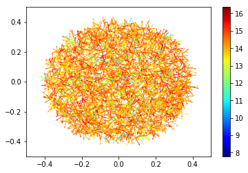
Let’s also look at the spatial distribution of the sites. To make the plot a little more interesting, we can also include the direction of the particle emitted from the source and color each source by the logarithm of its energy.
[26]:
plt.quiver(sp.source['r']['x'], sp.source['r']['y'],
           sp.source['u']['x'], sp.source['u']['y'],
           np.log(sp.source['E']), cmap='jet', scale=20.0)
plt.colorbar()
plt.xlim((-0.5,0.5))
plt.ylim((-0.5,0.5))
[26]:
(-0.5, 0.5)