4. Data Processing and Visualization

This section is intended to explain in detail the recommended procedures for carrying out common post-processing tasks with OpenMC. While several utilities of varying complexity are provided to help automate the process, the most powerful capabilities for post-processing derive from use of the Python API. Both the provided scripts and the Python API rely on a number third-party Python packages, including:

• [1] NumPy
• [2] h5py
• [3] pandas
• [4] matplotlib
• [4] Silomesh
• [4] VTK
• [4] lxml

Most of these are can easily be installed with pip or alternatively obtaining through a package manager.

[1]	Required for most post-processing tasks

[2]	Required for reading HDF5 output files

[3]	Optional dependency for advanced features in Python API

[4]	(1, 2, 3, 4) Not used directly by the Python API, but are optional dependencies for a number of scripts.

4.1. Geometry Visualization

Geometry plotting is carried out by creating a plots.xml, specifying plots, and running OpenMC with the –plot or -p command-line option (See Geometry Plotting Specification – plots.xml).

4.1.1. Plotting in 2D

See below for a simple example of a plots xml file that demonstrates the capabilities of 2D slice plots. Here we assume that there is a geometry.xml file containing 7 cells.

<?xml version="1.0" encoding="UTF-8"?>
<plots>

  <plot id="1" type="slice" color="cell" basis="xy">
      <filename> myplot </filename>
      <origin> 0 0 </origin>
      <width> 10 10 </width>
      <pixels> 2000 2000 </pixels>
      <background> 0 0 0 </background>
      <col_spec id="1" rgb="198 226 255"/>
      <col_spec id="2" rgb="255 218 185"/>
      <col_spec id="3" rgb="255 255 255"/>
      <col_spec id="4" rgb="101 101 101"/>
      <col_spec id="7" rgb="123 123 231"/>
      <mask background="255 255 255">
        <components> 1 3 4 5 6 </components>
      </mask>
  </plot>

</plots>

In this example, OpenMC will produce a plot named myplot.ppm when run in plotting mode. The picture will be on the xy-plane, depicting the rectangle between points (-5,-5) and (5,5) with 2000 pixels along each dimension. The color of each pixel is determined by placing a particle at the center of that pixel and using OpenMC’s internal find_cell routine (the same one used for particle tracking during simulation) to determine the cell and material at that location. In this example, pixels are 10/2000=0.005 cm wide, so points will be at (-4.9975,-4.9975), (-4.9950,-4.9975), (-4.9925,-4.9975), etc. This is pointed out to demonstrate that this plot may miss any features smaller than 0.005 cm, since they could exist between pixel centers. More pixels can be used to resolve finer features, but could result in larger files.

The background, col_spec, and mask elements define how to set pixel colors based on the cell ids at each pixel center. In this example, RGB colors are specified for cells 1,2,3,4, and 7, a random color will be assigned to cells 5 and 6, and a black background color (rgb="0 0 0") will be applied to locations where no cell is defined. However, the mask element here says that only cells 1,3,4,5, and 6 should be displayed, with other cells taking a white color (rgb="255 255 255"), which overrides the col_spec for cell 2 and the random color assigned to cell 7.

After running OpenMC to obtain PPM files, images should be saved to another format before using them elsewhere. This cuts down the size of the file by orders of magnitude. Most image viewers and editors that can view PPM images can also save to other formats (e.g. Gimp, IrfanView, etc.). However, more likely the user will want to convert to another format on the command line. This is easily accomplished with the convert command available on most Linux distributions as part of the ImageMagick package. (On Ubuntu: sudo apt-get install imagemagick). Images are then converted like:

convert myplot.ppm myplot.png

4.1.2. Plotting in 3D

See below for a simple example of a plots xml file that demonstrates the capabilities of 3D voxel plots.

<?xml version="1.0" encoding="UTF-8"?>
<plots>

  <plot id="1" type="voxel" color="mat">
      <filename> myplot </filename>
      <origin> 0 0 0 </origin>
      <width> 10 10 10 </width>
      <pixels> 500 500 500 </pixels>
  </plot>

</plots>

Voxel plots are built the same way 2D slice plots are, by determining the cell or material id of a particle at the center of each voxel. In this example, the space covered is the cube between the points (-5,-5,-5) and (5,5,5), with voxel centers 10/500 = 0.02 cm apart. The HDF5 voxel files that are produced do not specify any color - instead containing only material or cell ids (material id in this example) - and thus the background, col_spec, and mask elements are not used. If no cell is found at a voxel center, an id of -1 is stored.

The voxel plot data is written to an HDF5 file. The voxel file can subsequently be converted into a standard mesh format that can be viewed in ParaView, Visit, etc. This typically will compress the size of the file significantly. The provided utility openmc-voxel-to-silovtk accomplishes this for SILO:

openmc-voxel-to-silovtk myplot.voxel -o output.silo

and VTK file formats:

openmc-voxel-to-silovtk myplot.voxel --vtk -o output.vti

To use this utility you need either

• Silomesh

or

• VTK with python bindings. On debian derivatives, these are easily obtained with sudo apt-get install python-vtk

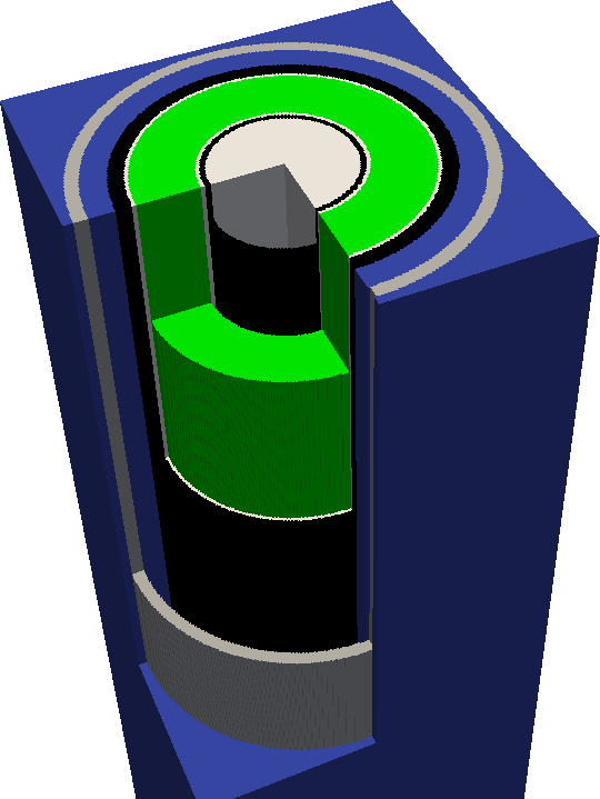
For the HDF5 file structure, see Voxel Plot File Format.

Once processed into a standard 3D file format, colors and masks can be defined using the stored id numbers to better explore the geometry. The process for doing this will depend on the 3D viewer, but should be straightforward.

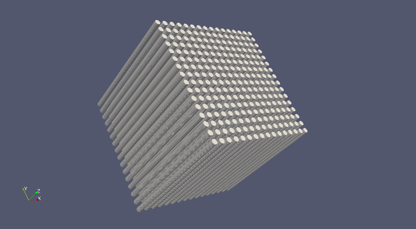
Note

3D voxel plotting can be very computer intensive for the viewing program (Visit, ParaView, etc.) if the number of voxels is large (>10 million or so). Thus if you want an accurate picture that renders smoothly, consider using only one voxel in a certain direction. For instance, the 3D pin lattice figure at the beginning of this section was generated with a 500x500x1 voxel mesh, which allows for resolution of the cylinders without wasting too many voxels on the axial dimension.

4.2. Tally Visualization

Tally results are saved in both a text file (tallies.out) as well as an HDF5 statepoint file. While the tallies.out file may be fine for simple tallies, in many cases the user requires more information about the tally or the run, or has to deal with a large number of result values (e.g. for mesh tallies). In these cases, extracting data from the statepoint file via the Python API is the preferred method of data analysis and visualization.

4.2.1. Data Extraction

A great deal of information is available in statepoint files (See State Point File Format), all of which is accessible through the Python API. The openmc.StatePoint class can load statepoints and access data as requested; it is used in many of the provided plotting utilities, OpenMC’s regression test suite, and can be used in user-created scripts to carry out manipulations of the data.

An example IPython notebook demonstrates how to extract data from a statepoint using the Python API.

4.2.2. Plotting in 2D

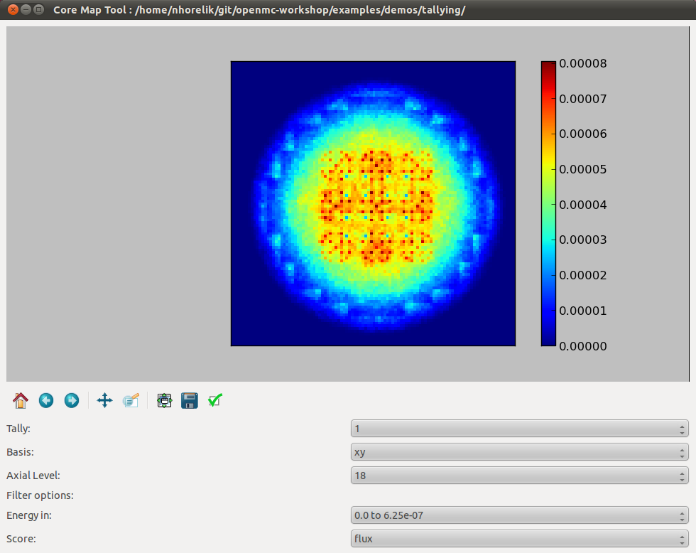
The IPython notebook example also demonstrates how to plot a mesh tally in two dimensions using the Python API. Note, however, that there is also a script distributed with OpenMC, openmc-plot-mesh-tally, that provides an interactive GUI to explore and plot mesh tallies for any scores and filter bins.

4.2.3. Plotting in 3D

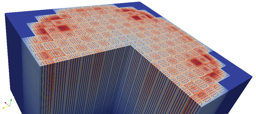
As with 3D plots of the geometry, meshtally data needs to be put into a standard format for viewing. The utility openmc-statepoint-3d is provided to accomplish this for both VTK and SILO. By default openmc-statepoint-3d processes a statepoint into a 3D file with all mesh tallies and filter/score combinations,

openmc-statepoint-3d <statepoint_file> -o output.silo
openmc-statepoint-3d <statepoint_file> --vtk -o output.vtm

but it also provides several command-line options to selectively process only certain data arrays in order to keep file sizes down.

openmc-statepoint-3d <statepoint_file> --tallies 2,4 --scores 4.1,4.3 -o output.silo
openmc-statepoint-3d <statepoint_file> --filters 2.energyin.1 --vtk -o output.vtm

All available options for specifying a subset of tallies, scores, and filters can be listed with the --list or -l command line options.

Note

Note that while SILO files can contain multiple meshes in one file, VTK needs to use a multi-block dataset, which stores each mesh piece in a different file in a subfolder. All meshes can be loaded at once with the main VTM file, or each VTI file in the subfolder can be loaded individually.

Alternatively, the user can write their own Python script to manipulate the data appropriately before insertion into a SILO or VTK file. For instance, if the data has been extracted as was done in the 2D plotting example script above, a SILO file can be created with:

import silomesh as sm
sm.init_silo("fluxtally.silo")
sm.init_mesh('tally_mesh', *mesh.dimension, *mesh.lower_left, *mesh.upper_right)
sm.init_var('flux_tally_thermal')
for x in range(1,nx+1):
  for y in range(1,ny+1):
      for z in range(1,nz+1):
        sm.set_value(float(thermal[(x,y,z)]),x,y,z)
sm.finalize_var()
sm.init_var('flux_tally_fast')
for x in range(1,nx+1):
  for y in range(1,ny+1):
      for z in range(1,nz+1):
          sm.set_value(float(fast[(x,y,z)]),x,y,z)
sm.finalize_var()
sm.finalize_mesh()
sm.finalize_silo()

and the equivalent VTK file with:

import vtk

grid = vtk.vtkImageData()
grid.SetDimensions(nx+1,ny+1,nz+1)
grid.SetOrigin(*mesh.lower_left)
grid.SetSpacing(*mesh.width)

# vtk cell arrays have x on the inners, so we need to reorder the data
idata = {}
for x in range(nx):
  for y in range(ny):
    for z in range(nz):
      i = z*nx*ny + y*nx + x
      idata[i] = (x,y,z)

vtkfastdata = vtk.vtkDoubleArray()
vtkfastdata.SetName("fast")
for i in range(nx*ny*nz):
  vtkfastdata.InsertNextValue(fast[idata[i]])

vtkthermaldata = vtk.vtkDoubleArray()
vtkthermaldata.SetName("thermal")
for i in range(nx*ny*nz):
  vtkthermaldata.InsertNextValue(thermal[idata[i]])

grid.GetCellData().AddArray(vtkfastdata)
grid.GetCellData().AddArray(vtkthermaldata)

writer = vtk.vtkXMLImageDataWriter()
writer.SetInput(grid)
writer.SetFileName('tally.vti')
writer.Write()

4.2.4. Getting Data into MATLAB

There is currently no front-end utility to dump tally data to MATLAB files, but the process is straightforward. First extract the data using the Python API via openmc.statepoint and then use the Scipy MATLAB IO routines to save to a MAT file. Note that all arrays that are accessible in a statepoint are already in NumPy arrays that can be reshaped and dumped to MATLAB in one step.

4.3. Particle Track Visualization

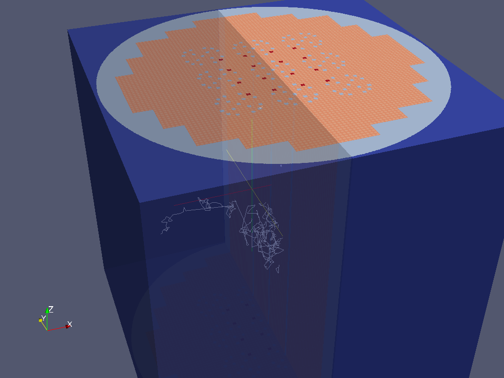
OpenMC can dump particle tracks—the position of particles as they are transported through the geometry. There are two ways to make OpenMC output tracks: all particle tracks through a command line argument or specific particle tracks through settings.xml.

Running OpenMC with the argument “-t”, “-track”, or “–track” will cause a track file to be created for every particle transported in the code.

The settings.xml file can dictate that specific particle tracks are output. These particles are specified within a ‘’track’’ element. The ‘’track’’ element should contain triplets of integers specifying the batch, generation, and particle numbers, respectively. For example, to output the tracks for particles 3 and 4 of batch 1 and generation 2 the settings.xml file should contain:

<track>
  1 2 3
  1 2 4
</track>

After running OpenMC, the directory should contain a file of the form “track_(batch #)_(generation #)_(particle #).h5” for each particle tracked. These track files can be converted into VTK poly data files with the openmc-track-to-vtk utility. The usage of openmc-track-to-vtk is of the form “openmc-track-to-vtk [-o OUT] IN” where OUT is the optional output filename and IN is one or more filenames describing track files. The default output name is “track.pvtp”. A common usage of track.py is “openmc-track-to-vtk track*.h5” which will use the data from all binary track files in the directory to write a “track.pvtp” VTK output file. The .pvtp file can then be read and plotted by 3d visualization programs such as ParaView.

4.4. Source Site Processing

For eigenvalue problems, OpenMC will store information on the fission source sites in the statepoint file by default. For each source site, the weight, position, sampled direction, and sampled energy are stored. To extract this data from a statepoint file, the openmc.statepoint module can be used. An example IPython notebook demontrates how to analyze and plot source information.