Using CAD-Based Geometries
In this notebook we’ll be exploring how to use CAD-based geometries in OpenMC via the DagMC toolkit. The models we’ll be using in this notebook have already been created using Trelis and faceted into a surface mesh represented as .h5m files in the Mesh Oriented DatABase format. We’ll be retrieving these files using the function below.
[1]:
import urllib.request

fuel_pin_url = 'https://tinyurl.com/y3ugwz6w' # 1.2 MB
teapot_url = 'https://tinyurl.com/y4mcmc3u' # 29 MB

def download(url):
    """
    Helper function for retrieving dagmc models
    """
    u = urllib.request.urlopen(url)

    if u.status != 200:
        raise RuntimeError("Failed to download file.")

    # save file as dagmc.h5m
    with open("dagmc.h5m", 'wb') as f:
        f.write(u.read())
This notebook is intended to demonstrate how DagMC problems are run in OpenMC. For more information on how DagMC models are created, please refer to the DagMC User’s Guide.
[2]:
%matplotlib inline
from IPython.display import Image
import openmc
To start, we’ll be using a simple U235 fuel pin surrounded by a water moderator, so let’s create those materials.
[3]:
 # materials
u235 = openmc.Material(name="fuel")
u235.add_nuclide('U235', 1.0, 'ao')
u235.set_density('g/cc', 11)
u235.id = 40

water = openmc.Material(name="water")
water.add_nuclide('H1', 2.0, 'ao')
water.add_nuclide('O16', 1.0, 'ao')
water.set_density('g/cc', 1.0)
water.add_s_alpha_beta('c_H_in_H2O')
water.id = 41

mats = openmc.Materials([u235, water])
mats.export_to_xml()
Now let’s get our DAGMC geometry. We’ll be using prefabricated models in this notebook. For information on how to create your own DAGMC models, you can refer to the instructions here.
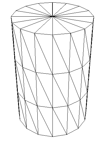
Let’s download the DAGMC model. These models come in the form of triangle surface meshes stored using the the Mesh Oriented datABase (MOAB) in an HDF5 file with the extension .h5m. An example of a coarse triangle mesh looks like:
[4]:
Image("./images/cylinder_mesh.png", width=350)
[4]:
First we’ll need to grab some pre-made DagMC models.
[5]:
download(fuel_pin_url)
OpenMC expects that the model has the name “dagmc.h5m” so we’ll name the file that and indicate to OpenMC that a DAGMC geometry is being used by setting the settings.dagmc attribute to True.
[6]:
settings = openmc.Settings()
settings.dagmc = True
settings.batches = 10
settings.inactive = 2
settings.particles = 5000
settings.export_to_xml()
Unlike conventional geometries in OpenMC, we really have no way of knowing what our model looks like at this point. Thankfully DagMC geometries can be plotted just like any other OpenMC geometry to give us an idea of what we’re now working with.
Note that material assignments have already been applied to this model. Materials can be assigned either using ids or names of materials in the materials.xml file. It is recommended that material names are used for assignment for readability.
[7]:
p = openmc.Plot()
p.width = (25.0, 25.0)
p.pixels = (400, 400)
p.color_by = 'material'
p.colors = {u235: 'yellow', water: 'blue'}
openmc.plot_inline(p)

Now that we’ve had a chance to examine the model a bit, we can finish applying our settings and add a source.
[8]:
settings.source = openmc.Source(space=openmc.stats.Box([-4., -4., -4.],
                                                       [ 4.,  4.,  4.]))
settings.export_to_xml()
Tallies work in the same way when using DAGMC geometries too. We’ll add a tally on the fuel cell here.
[9]:
tally = openmc.Tally()
tally.scores = ['total']
tally.filters = [openmc.CellFilter(1)]
tallies = openmc.Tallies([tally])
tallies.export_to_xml()
Note: Applying tally filters in DagMC models requires prior knowledge of the model. Here, we know that the fuel cell’s volume ID in the CAD sofware is 1. To identify cells without use of CAD software, load them into the OpenMC plotter where cell, material, and volume IDs can be identified for native both OpenMC and DagMC geometries.
Now we’re ready to run the simulation just like any other OpenMC run.
[10]:
openmc.run()
                                %%%%%%%%%%%%%%%
                           %%%%%%%%%%%%%%%%%%%%%%%%
                        %%%%%%%%%%%%%%%%%%%%%%%%%%%%%%
                      %%%%%%%%%%%%%%%%%%%%%%%%%%%%%%%%%%
                    %%%%%%%%%%%%%%%%%%%%%%%%%%%%%%%%%%%%%%
                   %%%%%%%%%%%%%%%%%%%%%%%%%%%%%%%%%%%%%%%%
                                    %%%%%%%%%%%%%%%%%%%%%%%%
                                     %%%%%%%%%%%%%%%%%%%%%%%%
                 ###############      %%%%%%%%%%%%%%%%%%%%%%%%
                ##################     %%%%%%%%%%%%%%%%%%%%%%%
                ###################     %%%%%%%%%%%%%%%%%%%%%%%
                ####################     %%%%%%%%%%%%%%%%%%%%%%
                #####################     %%%%%%%%%%%%%%%%%%%%%
                ######################     %%%%%%%%%%%%%%%%%%%%
                #######################     %%%%%%%%%%%%%%%%%%
                 #######################     %%%%%%%%%%%%%%%%%
                 ######################     %%%%%%%%%%%%%%%%%
                  ####################     %%%%%%%%%%%%%%%%%
                    #################     %%%%%%%%%%%%%%%%%
                     ###############     %%%%%%%%%%%%%%%%
                       ############     %%%%%%%%%%%%%%%
                          ########     %%%%%%%%%%%%%%
                                      %%%%%%%%%%%

                   | The OpenMC Monte Carlo Code
         Copyright | 2011-2019 MIT and OpenMC contributors
           License | http://openmc.readthedocs.io/en/latest/license.html
           Version | 0.11.0-dev
          Git SHA1 | 2c0b16e73d5d81a2f849f4e2bfae5eb5319f2417
         Date/Time | 2019-06-18 08:54:17
    OpenMP Threads | 2

 Reading settings XML file...
 Reading cross sections XML file...
 Reading materials XML file...
 Reading DAGMC geometry...
Loading file dagmc.h5m
Initializing the GeomQueryTool...
Using faceting tolerance: 0.0001
Building OBB Tree...
 Reading U235 from /home/shriwise/opt/openmc/xs/nndc_hdf5/U235.h5
 Reading H1 from /home/shriwise/opt/openmc/xs/nndc_hdf5/H1.h5
 Reading O16 from /home/shriwise/opt/openmc/xs/nndc_hdf5/O16.h5
 Reading c_H_in_H2O from /home/shriwise/opt/openmc/xs/nndc_hdf5/c_H_in_H2O.h5
 Maximum neutron transport energy: 20000000.000000 eV for U235
 Reading tallies XML file...
 Writing summary.h5 file...
 Initializing source particles...

 ====================>     K EIGENVALUE SIMULATION     <====================

  Bat./Gen.      k            Average k
  =========   ========   ====================
        1/1    1.15789
        2/1    1.05169
        3/1    1.00736
        4/1    0.97863    0.99300 +/- 0.01436
        5/1    0.95316    0.97972 +/- 0.01566
        6/1    0.95079    0.97248 +/- 0.01322
        7/1    0.96879    0.97175 +/- 0.01027
        8/1    0.94253    0.96688 +/- 0.00970
        9/1    0.97406    0.96790 +/- 0.00826
       10/1    0.97362    0.96862 +/- 0.00719
 Creating state point statepoint.10.h5...

 =======================>     TIMING STATISTICS     <=======================

 Total time for initialization     = 2.4575e-01 seconds
   Reading cross sections          = 1.3129e-01 seconds
 Total time in simulation          = 1.6897e+00 seconds
   Time in transport only          = 1.6829e+00 seconds
   Time in inactive batches        = 3.1605e-01 seconds
   Time in active batches          = 1.3737e+00 seconds
   Time synchronizing fission bank = 2.8739e-03 seconds
     Sampling source sites         = 2.5550e-03 seconds
     SEND/RECV source sites        = 2.8512e-04 seconds
   Time accumulating tallies       = 7.8450e-06 seconds
 Total time for finalization       = 1.7404e-04 seconds
 Total time elapsed                = 1.9588e+00 seconds
 Calculation Rate (inactive)       = 31640.8 particles/second
 Calculation Rate (active)         = 29119.1 particles/second

 ============================>     RESULTS     <============================

 k-effective (Collision)     = 0.97020 +/- 0.00750
 k-effective (Track-length)  = 0.96862 +/- 0.00719
 k-effective (Absorption)    = 0.95742 +/- 0.00791
 Combined k-effective        = 0.96203 +/- 0.00898
 Leakage Fraction            = 0.57677 +/- 0.00317
More Complicated Geometry
Neat! But this pincell is something we could’ve done with CSG. Let’s take a look at something more complex. We’ll download a pre-built model of the Utah teapot and use it here.
[11]:
download(teapot_url)
[12]:
Image("./images/teapot.jpg", width=600)
[12]:

Our teapot is made out of iron, so we’ll want to create that material and make sure it is in our materials.xml file.
[13]:
iron = openmc.Material(name="iron")
iron.add_nuclide("Fe54", 0.0564555822608)
iron.add_nuclide("Fe56", 0.919015287728)
iron.add_nuclide("Fe57", 0.0216036861685)
iron.add_nuclide("Fe58", 0.00292544384231)
iron.set_density("g/cm3", 7.874)
mats = openmc.Materials([iron, water])
mats.export_to_xml()
To make sure we’ve updated the file correctly, let’s make a plot of the teapot.
[14]:
p = openmc.Plot()
p.basis = 'xz'
p.origin = (0.0, 0.0, 0.0)
p.width = (30.0, 20.0)
p.pixels = (450, 300)
p.color_by = 'material'
p.colors = {iron: 'gray', water: 'blue'}
openmc.plot_inline(p)
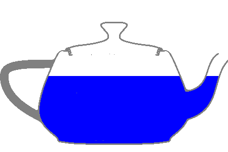
Here we start to see some of the advantages CAD geometries provide. This particular file was pulled from the GrabCAD and pushed through the DAGMC workflow without modification (other than the addition of material assignments). It would take a considerable amount of time to create a model like this using CSG!
[15]:
p.width = (18.0, 6.0)
p.basis = 'xz'
p.origin = (10.0, 0.0, 5.0)
p.pixels = (600, 200)
p.color_by = 'material'
openmc.plot_inline(p)

Now let’s brew some tea! … using a very hot neutron source. We’ll use some well-placed point sources distributed throughout the model.
[16]:
settings = openmc.Settings()
settings.dagmc = True
settings.batches = 10
settings.particles = 5000
settings.run_mode = "fixed source"

src_locations = ((-4.0, 0.0, -2.0),
                 ( 4.0, 0.0, -2.0),
                 ( 4.0, 0.0, -6.0),
                 (-4.0, 0.0, -6.0),
                 (10.0, 0.0, -4.0),
                 (-8.0, 0.0, -4.0))

# we'll use the same energy for each source
src_e = openmc.stats.Discrete(x=[12.0,], p=[1.0,])

# create source for each location
sources = []
for loc in src_locations:
    src_pnt = openmc.stats.Point(xyz=loc)
    src = openmc.Source(space=src_pnt, energy=src_e)
    sources.append(src)

src_str = 1.0 / len(sources)
for source in sources:
    source.strength = src_str

settings.source = sources
settings.export_to_xml()
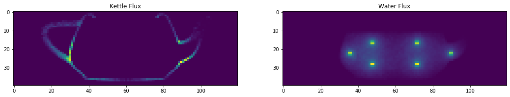
…and setup a couple mesh tallies. One for the kettle, and one for the water inside.
[17]:
mesh = openmc.RegularMesh()
mesh.dimension = (120, 1, 40)
mesh.lower_left = (-20.0, 0.0, -10.0)
mesh.upper_right = (20.0, 1.0, 4.0)

mesh_filter = openmc.MeshFilter(mesh)

pot_filter = openmc.CellFilter([1])
pot_tally = openmc.Tally()
pot_tally.filters = [mesh_filter, pot_filter]
pot_tally.scores = ['flux']

water_filter = openmc.CellFilter([5])
water_tally = openmc.Tally()
water_tally.filters = [mesh_filter, water_filter]
water_tally.scores = ['flux']


tallies = openmc.Tallies([pot_tally, water_tally])
tallies.export_to_xml()
[18]:
openmc.run()
                                %%%%%%%%%%%%%%%
                           %%%%%%%%%%%%%%%%%%%%%%%%
                        %%%%%%%%%%%%%%%%%%%%%%%%%%%%%%
                      %%%%%%%%%%%%%%%%%%%%%%%%%%%%%%%%%%
                    %%%%%%%%%%%%%%%%%%%%%%%%%%%%%%%%%%%%%%
                   %%%%%%%%%%%%%%%%%%%%%%%%%%%%%%%%%%%%%%%%
                                    %%%%%%%%%%%%%%%%%%%%%%%%
                                     %%%%%%%%%%%%%%%%%%%%%%%%
                 ###############      %%%%%%%%%%%%%%%%%%%%%%%%
                ##################     %%%%%%%%%%%%%%%%%%%%%%%
                ###################     %%%%%%%%%%%%%%%%%%%%%%%
                ####################     %%%%%%%%%%%%%%%%%%%%%%
                #####################     %%%%%%%%%%%%%%%%%%%%%
                ######################     %%%%%%%%%%%%%%%%%%%%
                #######################     %%%%%%%%%%%%%%%%%%
                 #######################     %%%%%%%%%%%%%%%%%
                 ######################     %%%%%%%%%%%%%%%%%
                  ####################     %%%%%%%%%%%%%%%%%
                    #################     %%%%%%%%%%%%%%%%%
                     ###############     %%%%%%%%%%%%%%%%
                       ############     %%%%%%%%%%%%%%%
                          ########     %%%%%%%%%%%%%%
                                      %%%%%%%%%%%

                   | The OpenMC Monte Carlo Code
         Copyright | 2011-2019 MIT and OpenMC contributors
           License | http://openmc.readthedocs.io/en/latest/license.html
           Version | 0.11.0-dev
          Git SHA1 | 2c0b16e73d5d81a2f849f4e2bfae5eb5319f2417
         Date/Time | 2019-06-18 08:54:35
    OpenMP Threads | 2

 Reading settings XML file...
 Reading cross sections XML file...
 Reading materials XML file...
 Reading DAGMC geometry...
Loading file dagmc.h5m
Initializing the GeomQueryTool...
Using faceting tolerance: 0.001
Building OBB Tree...
 Reading Fe54 from /home/shriwise/opt/openmc/xs/nndc_hdf5/Fe54.h5
 Reading Fe56 from /home/shriwise/opt/openmc/xs/nndc_hdf5/Fe56.h5
 Reading Fe57 from /home/shriwise/opt/openmc/xs/nndc_hdf5/Fe57.h5
 Reading Fe58 from /home/shriwise/opt/openmc/xs/nndc_hdf5/Fe58.h5
 Reading H1 from /home/shriwise/opt/openmc/xs/nndc_hdf5/H1.h5
 Reading O16 from /home/shriwise/opt/openmc/xs/nndc_hdf5/O16.h5
 Reading c_H_in_H2O from /home/shriwise/opt/openmc/xs/nndc_hdf5/c_H_in_H2O.h5
 Maximum neutron transport energy: 20000000.000000 eV for Fe58
 Reading tallies XML file...
 Writing summary.h5 file...
 Initializing source particles...

 ===============>     FIXED SOURCE TRANSPORT SIMULATION     <===============

 Simulating batch 1
 Simulating batch 2
 Simulating batch 3
 Simulating batch 4
 Simulating batch 5
 Simulating batch 6
 Simulating batch 7
 Simulating batch 8
 Simulating batch 9
 Simulating batch 10
 Creating state point statepoint.10.h5...

 =======================>     TIMING STATISTICS     <=======================

 Total time for initialization     = 4.9659e+00 seconds
   Reading cross sections          = 6.3783e-01 seconds
 Total time in simulation          = 1.5112e+01 seconds
   Time in transport only          = 1.4102e+01 seconds
   Time in active batches          = 1.5112e+01 seconds
   Time accumulating tallies       = 2.8790e-04 seconds
 Total time for finalization       = 3.2375e-02 seconds
 Total time elapsed                = 2.0224e+01 seconds
 Calculation Rate (active)         = 3308.59 particles/second

 ============================>     RESULTS     <============================

 Leakage Fraction            = 0.62594 +/- 0.00117
Note that the performance is significantly lower than our pincell model due to the increased complexity of the model, but it allows us to examine tally results like these:
[19]:
sp = openmc.StatePoint("statepoint.10.h5")

water_tally = sp.get_tally(scores=['flux'], id=water_tally.id)
water_flux = water_tally.mean
water_flux.shape = (40, 120)
water_flux = water_flux[::-1, :]

pot_tally = sp.get_tally(scores=['flux'], id=pot_tally.id)
pot_flux = pot_tally.mean
pot_flux.shape = (40, 120)
pot_flux = pot_flux[::-1, :]

del sp
[20]:
from matplotlib import pyplot as plt
fig = plt.figure(figsize=(18, 16))

sub_plot1 = plt.subplot(121, title="Kettle Flux")
sub_plot1.imshow(pot_flux)

sub_plot2 = plt.subplot(122, title="Water Flux")
sub_plot2.imshow(water_flux)
[20]:
<matplotlib.image.AxesImage at 0x7f90d12b8198>